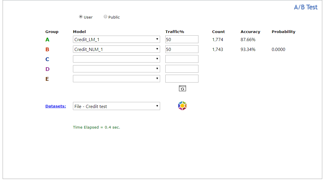
Explorer - Univariate
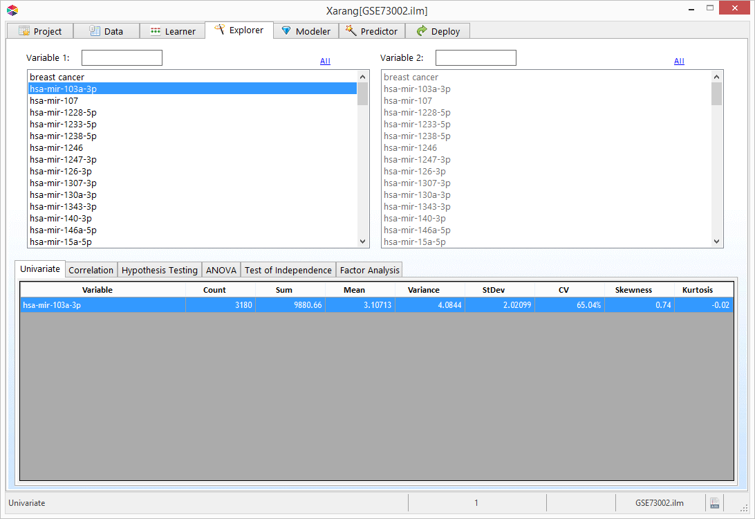
Univariate data analysis explores attributes (variables) one by one using statistical analysis. Attributes are either numerical or categorical (encoded to binary). Learn more
- Select the Univariate tab.
- Select one or more variables from the Variable 1 list.
- To view only Binary or Numeric variables, click All, then Binary or Numeric.
Explorer - Bivariate
Bivariate analysis is the simultaneous analysis of two variables (attributes).
It explores the concept of relationship between two variables, whether there exists an association and the
strength of this association, or whether there are differences between two variables and the significance of
these differences. There are four types of bivariate analysis.
- Correlation
- Hypothesis Testing
- ANOVA
- Test of Independence
Correlation
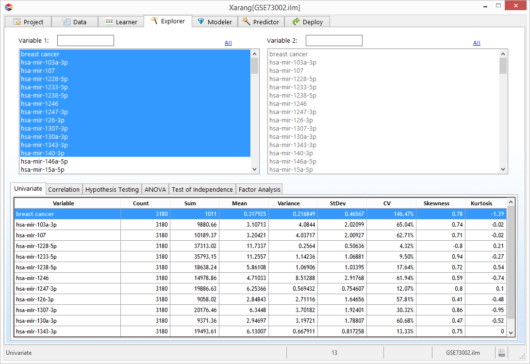
Linear correlation quantifies the strength of a linear relationship between two numerical variables.
When there is no correlation between two variables, there is no tendency for the values of one quantity to
increase or decrease with the values of the second quantity. Learn more
- Select the Correlation tab.
- Select one or more variables from the Variable 1 list.
- Select the second variable from the Variable 2 list.
- Click
 to visualize the result.
Hypothesis Testing
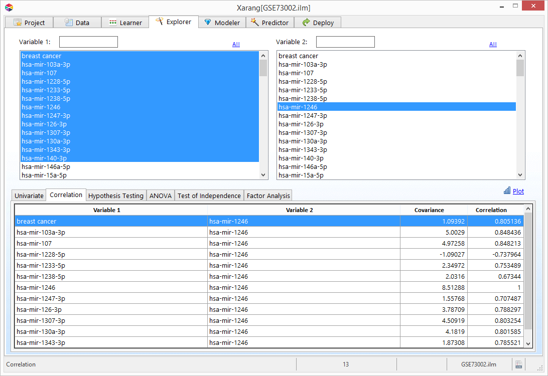
- Select the Hypothesis Testing tab.
- Select a numerical variable from the Variable 2 list. Note: To view only Binary or Numeric variables, click All, then Binary or Numeric.
- Select Binary Variable 1 and if necessary Binary Variable 2 from the drop down lists.
- Click Z Test , T Test , or F Test button. The related result will be displayed.
- Click
 to visualize the result.
Z Test
The Z test assesses whether the difference between averages of two attributes are statistically significant.
This analysis is appropriate for comparing the average of a numerical attribute with a known average or
two conditional averages of a numerical attribute given two binary attributes (two categories of the same categorical attribute).
Learn more
T Test
The T test like Z test assesses whether the averages of two numerical attributes are statistically different
from each other when the number of data points is less than 30. T test is appropriate for comparing the average
of a numerical attribute with a known average or two conditional averages of a numerical attribute given two
binary attributes (two categories of the same categorical attribute).
Learn more
F Test
The F-test is used to compare the variances of two attributes.F test can be used for comparing the variance of a numerical \
attribute with a known variance or two conditional variances of a numerical attribute given two binary attributes
(two categories of the same categorical attribute).
Learn more
ANOVA
ANOVA (Analysis of Variance) assesses whether the averages of more than two groups are statistically different
from each other, under the assumption that the corresponding populations are normally distributed. ANOVA is useful
for comparing averages of two or more numerical attributes or two or more conditional averages of a numerical
attribute given two or more binary attributes (two or more categories of the same categorical attribute).
Learn more
- Select the ANOVA tab.
- Select a numerical variable from the Variable 2 list. Note: To view only Binary or Numeric variables, click All, then Binary or Numeric.
- Select the Binary Variables from the Binary Variables list.
- Click the ANOVA button. The ANOVA table will be displayed.
- Click the Stats radio button to view the Count, Mean, and Variance.
- Click
 to visualize the result.

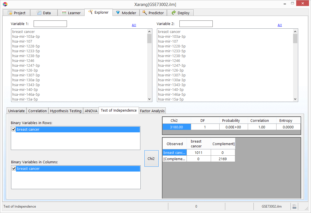
Test of Independence
The Chi2 test can be used to determine the association between categorical (binary) attributes. It is based on the
difference between the expected frequencies and the observed frequencies in one or more categories in the frequency
table. The Chi2 distribution returns a probability for the computed Chi2 and the degree of freedom. A probability
of zero shows complete dependency between two categorical attributes and a probability of one means that two
categorical attributes are completely independent.Learn more
- Select the Test of Independence tab.
- Select Binary variables in Rows and a Binary variables in Columns.
- Click the Chi2 button.
Explorer - Factor Analysis
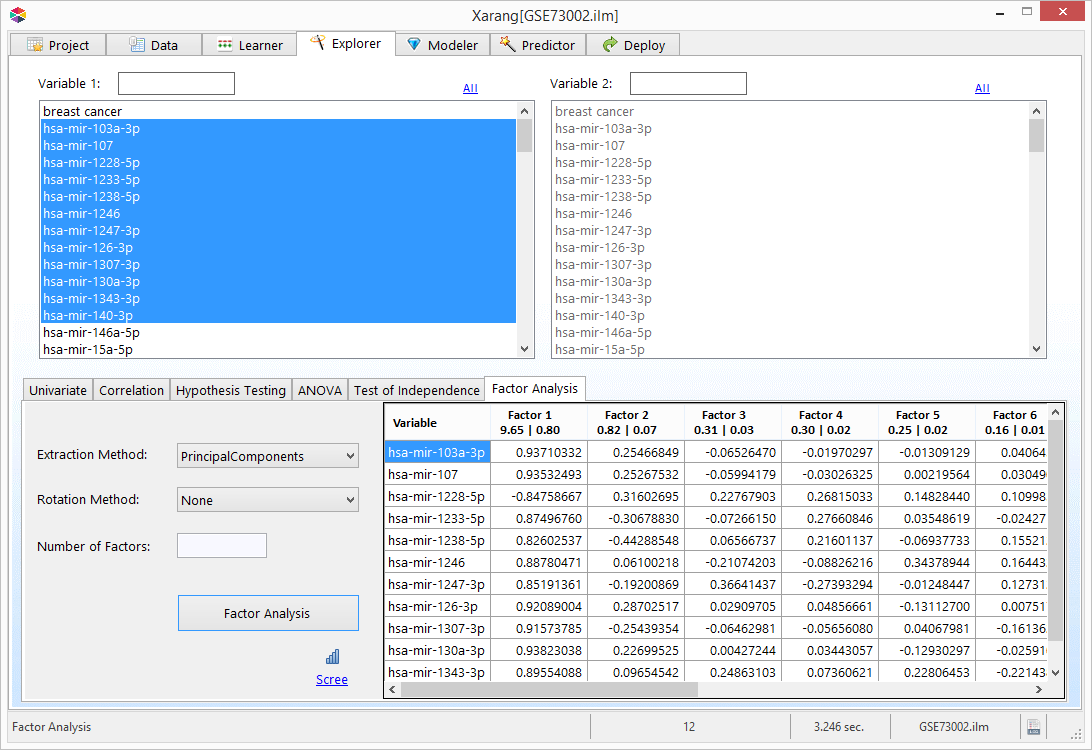
Factor analysis is a statistical method used to describe variability among observed, correlated variables in terms
of a potentially lower number of unobserved variables called factors. For example, people may respond similarly to
questions about income, education, and occupation, which are all associated with the latent variable socioeconomic
status. The relationship of each variable to the underlying factor is expressed by the so-called factor loading.
Here is an example of the output of a simple factor analysis. The first number underneath of every factor are
"eigenvalue" and "percentage of variance explained".
Extraction Methods:
Xarang supports six extraction methods:
- Alpha Factoring
- Generalized Least Squares
- Image Factoring
- Iterative Principal Axis
- Maximum Likelihood
- Principal Components Analysis (PCA)
- Unweighted Least Squares
PCA is the most popular extraction method. However, information on the relative strengths and weaknesses of these techniques is not
well known. In general, Maximum Likelihood or Iterative Principal Axis will give you the best results,depending on whether your data
are generally normally-distributed or significantly non-normal, respectively.
Number of Factors:
After extraction you must decide how many factors to retain for rotation. Both over-extraction and under-extraction
of factors retained for rotation can have damaging effects on the results. The default in most statistical software
packages is to retain all factors with eigenvalues greater than 1.0. Alternate tests for factor retention include
the screen test. The scree test involves examining the graph of the eigenvalues and looking for the natural bend or
break point in the data where the curve flattens out. The number of datapoints above the “break”
(i.e., not including the point at which the break occurs) is usually the number of factors to retain.
Rotation Methods:
An important feature of factor analysis is that the axes of the factors can be rotated within the multidimensional
variable space. Rotations that allow for correlation are called oblique rotations; rotations that assume the factors
are not correlated are called orthogonal rotations.
Varimax is the most popular orthogonal rotation and Promax is the only oblique rotation method supported by Xarang.
- Equamax
- Promax
- Quartimax
- Varimax
Predictor - Data
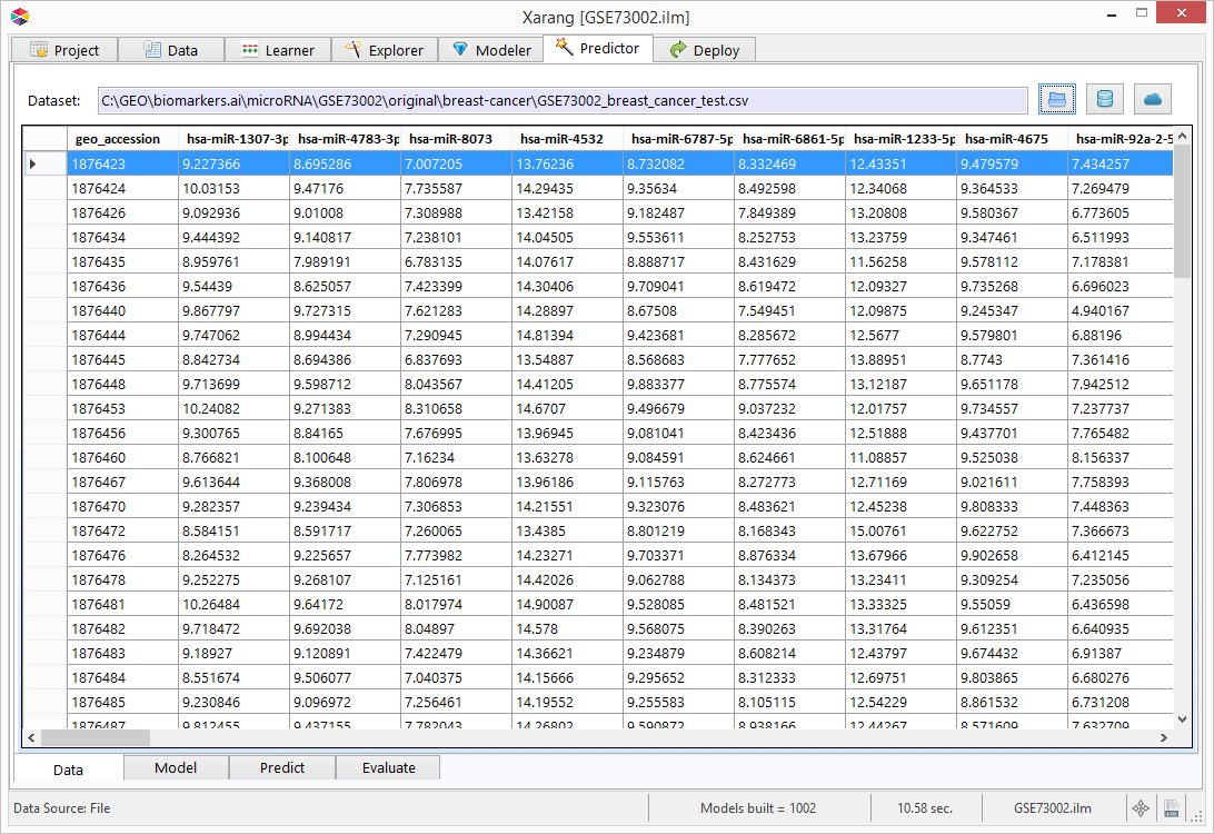
On the Predictor tab opens to the Data tab. Load the dataset from a local drive, a database or a Cloud service that
you would like to use to make predictions.
Predictor - Model
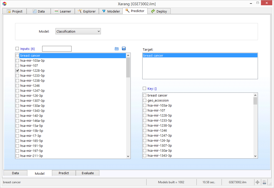
- Click the Model tab.
- Select either Classification, Regression or MultiCLass from the Model drop-down list.
- Select one or more Input variables and a Target variable.
- You can also append other variables to the output file by selecting them from the Key list.
Predictor - Predict
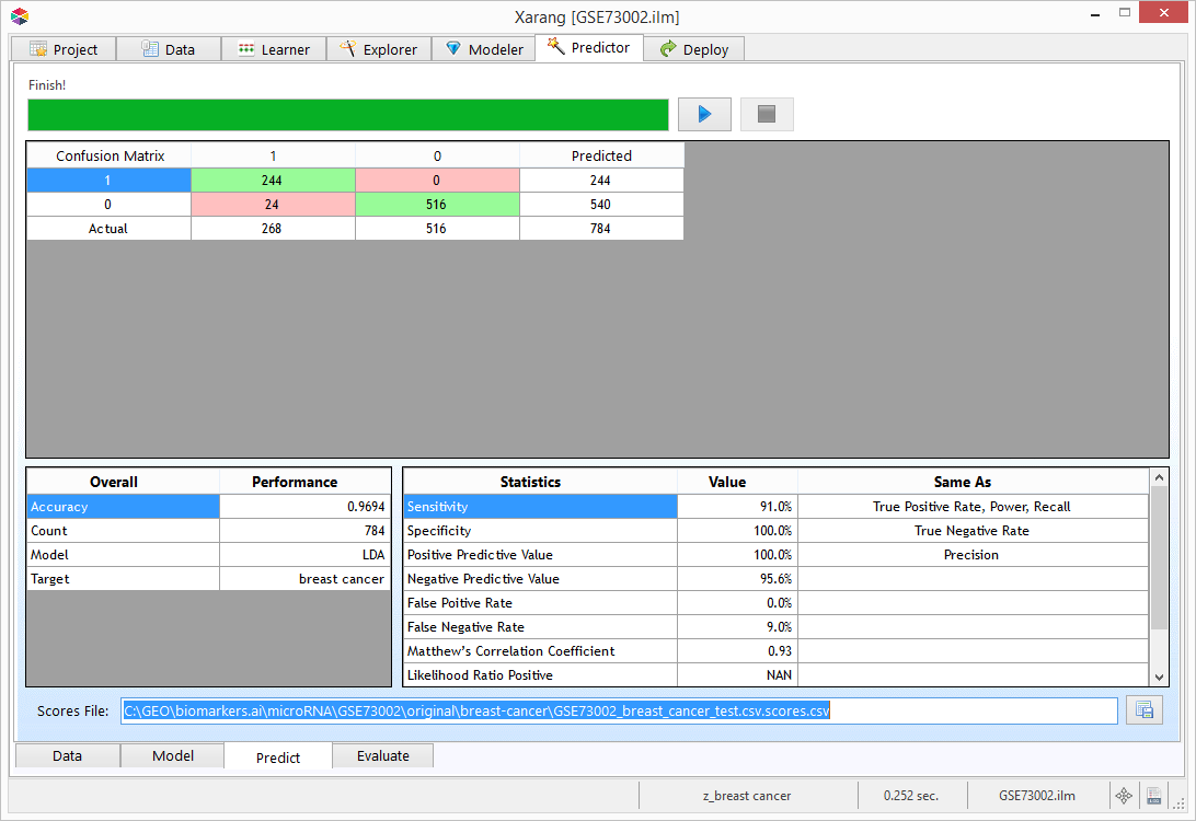
To begin the Predictor, click the Start Predictor button. The results will be displayed and an output file will be
created. Learn more about LDA,
MLR and
model evaluation
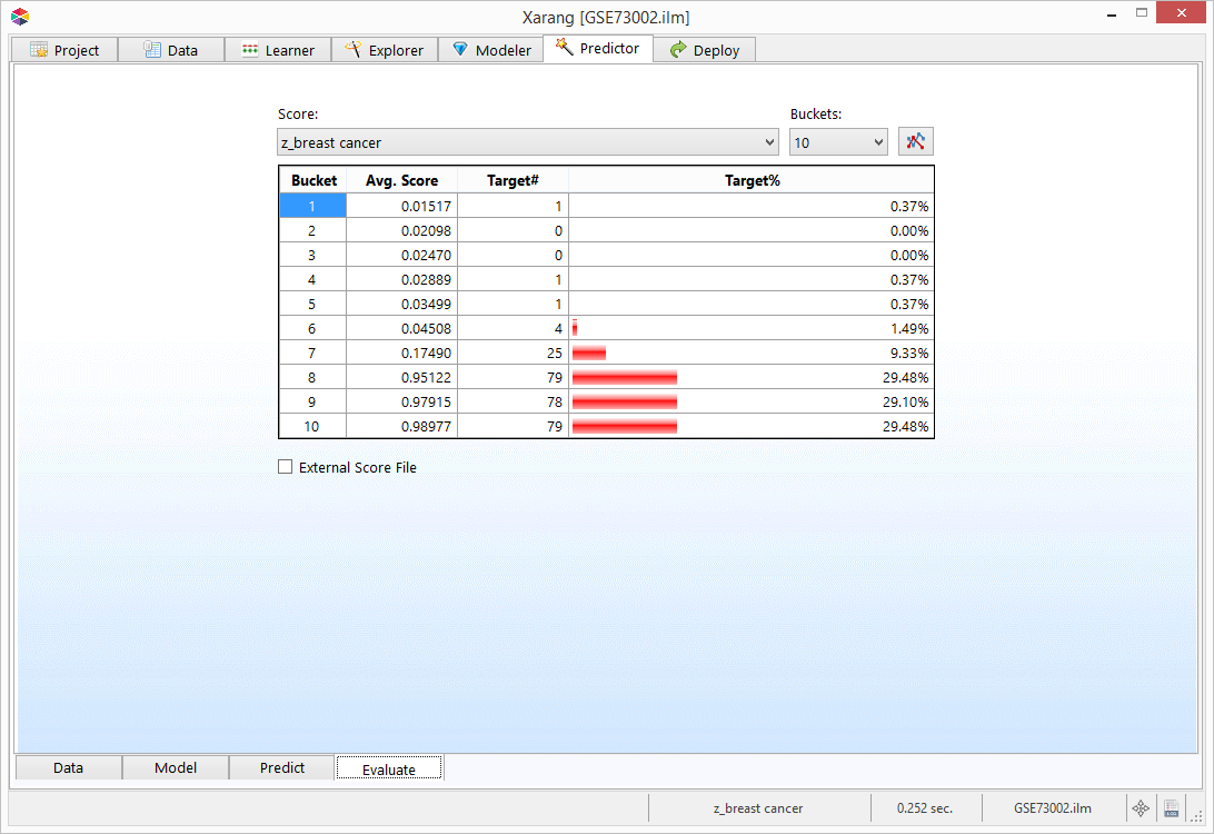
Predictor - Evaluate
If you have used a Classification Model, click on  to view more evaluation charts.
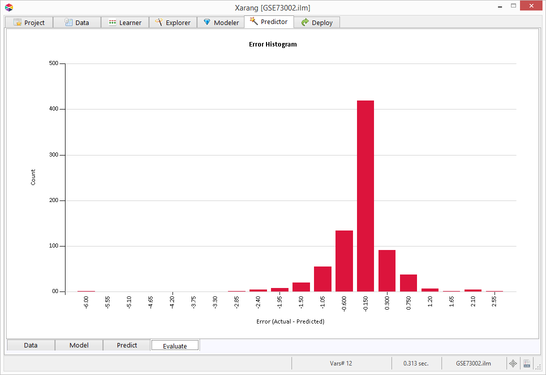
This is Error Histogram for a regression model.
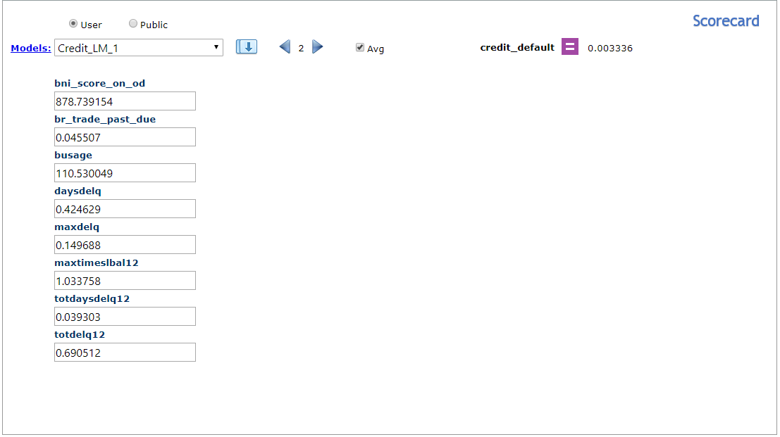
Scorecard
- Click "Models" to refresh the list.
- Select a model from the list and click
 .
.
- Fill the scorecard or check "Avg" to fill the scorecard with the related average values.
- Click
 to predict using the model.
- Click
 or
or  to browse the current session queries.



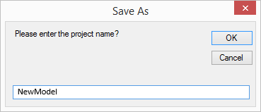

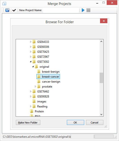
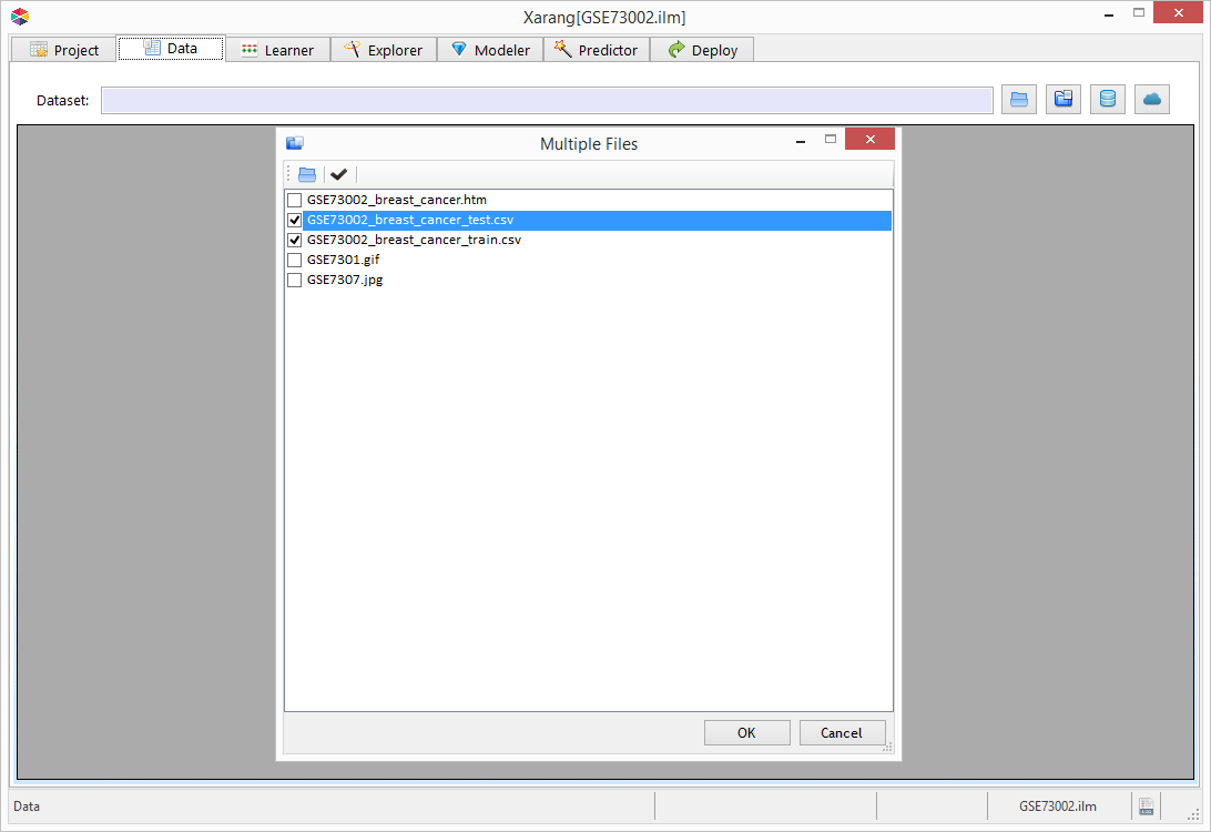
 to open "Browse For Folder" dialogue box.
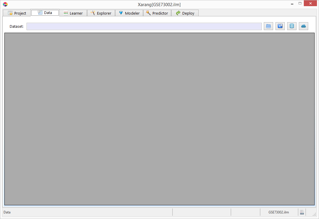
 button.
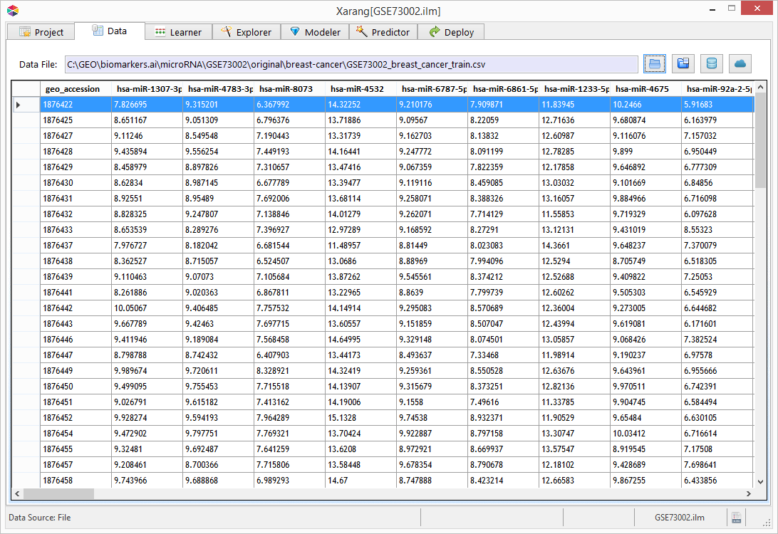
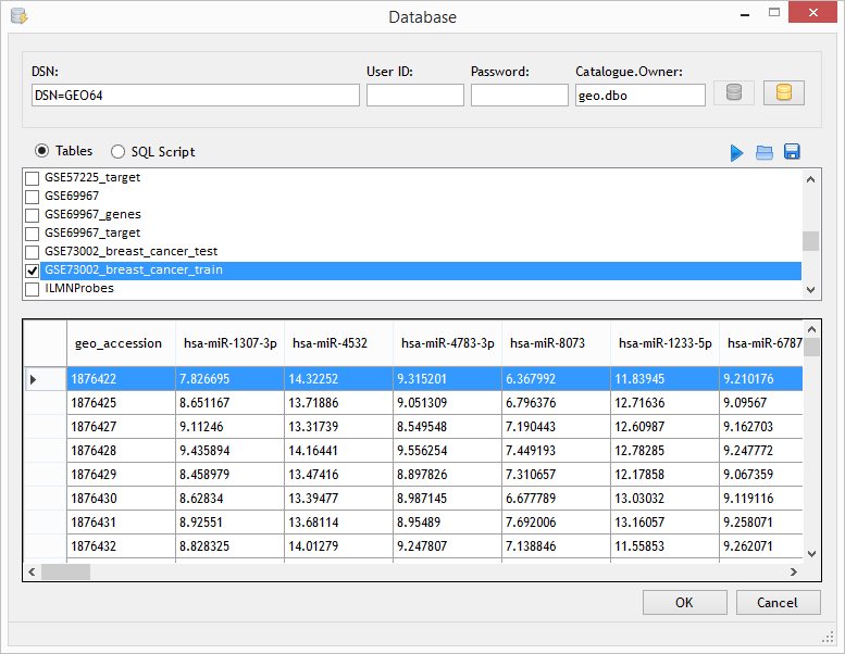
 button.

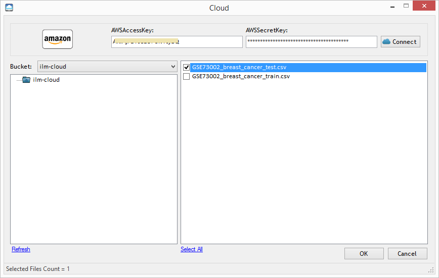
 to guess the type of each variable. You can change the type of variable by right clicking on that variable.
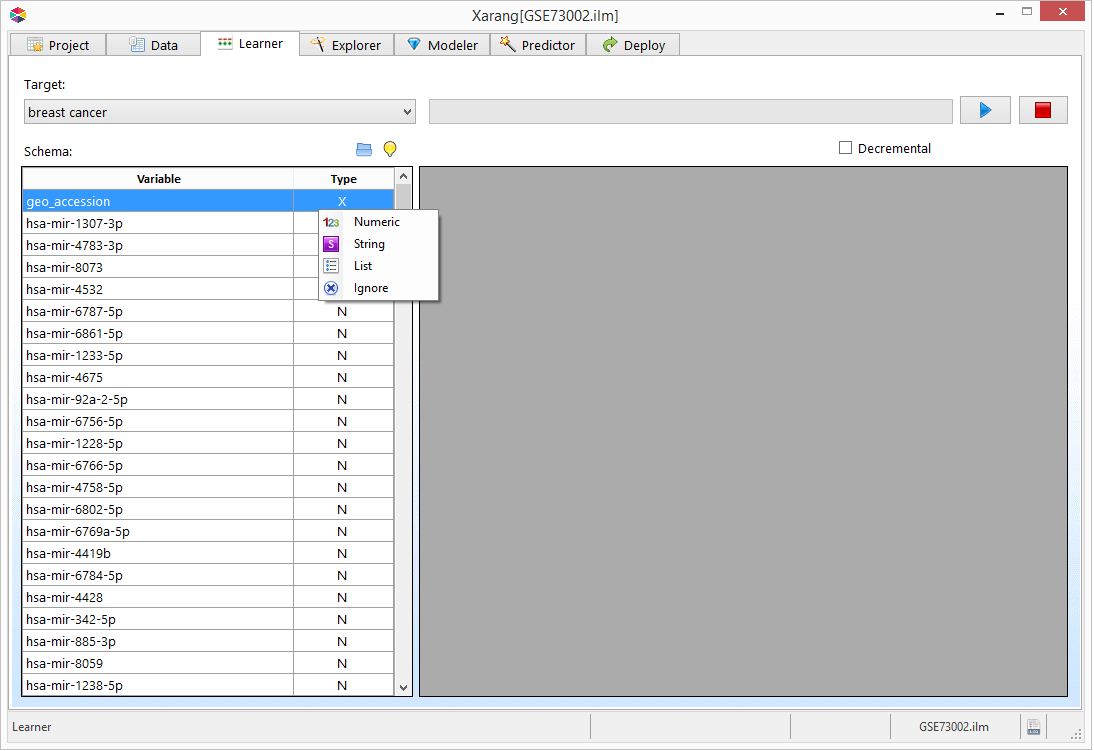
 .
.
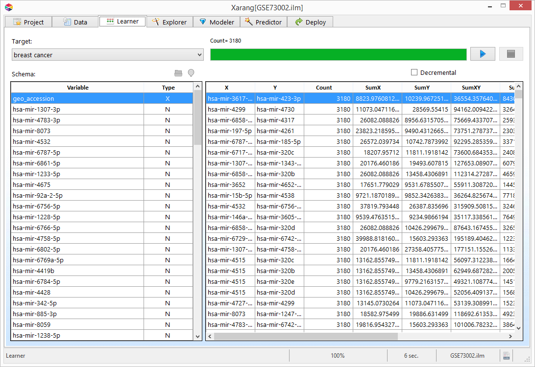
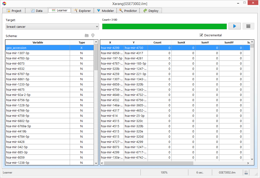

 to visualize the result.


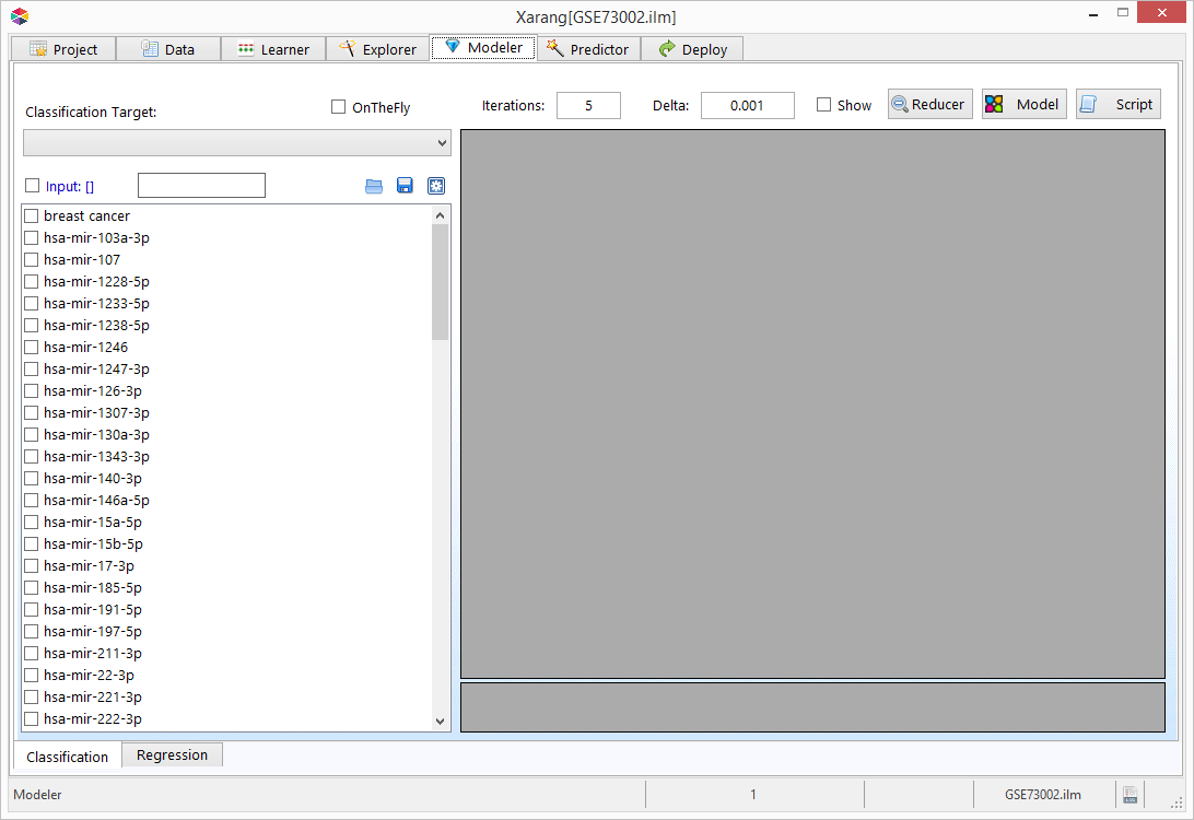
 to save the selected variables.
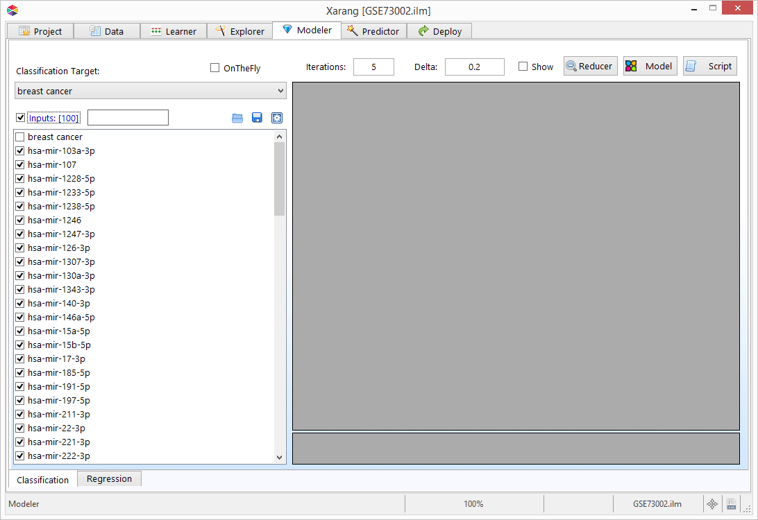
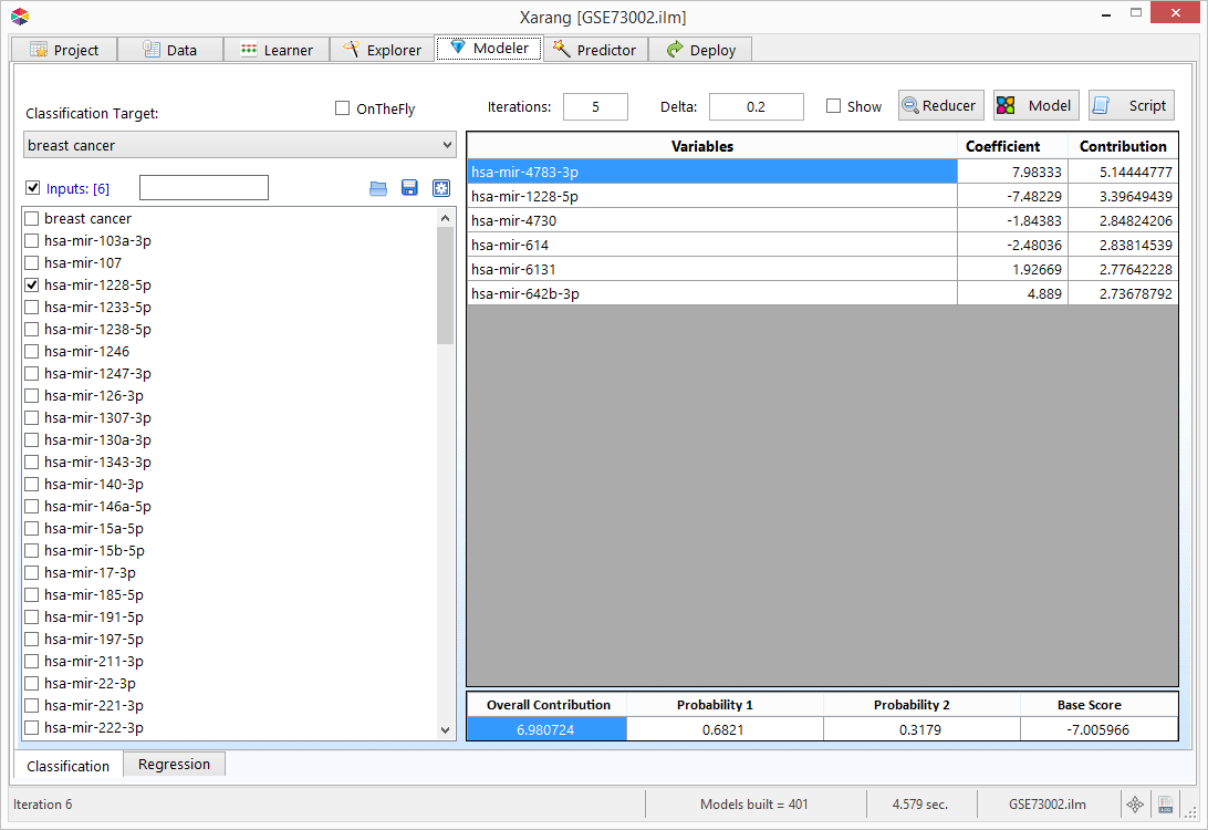
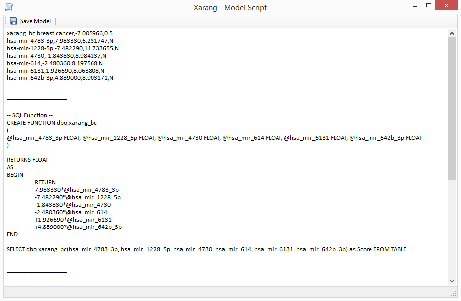
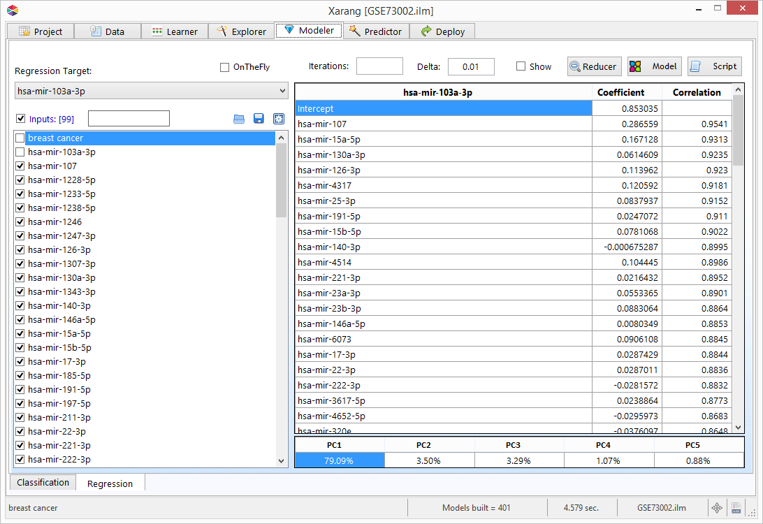
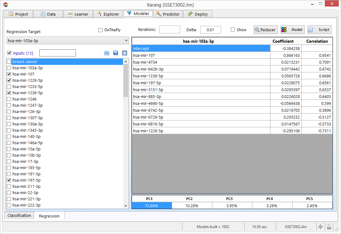
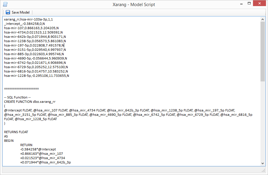
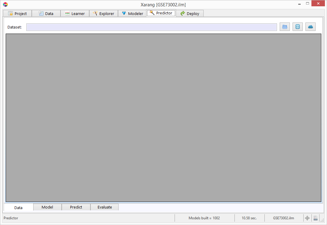


 to view more evaluation charts.

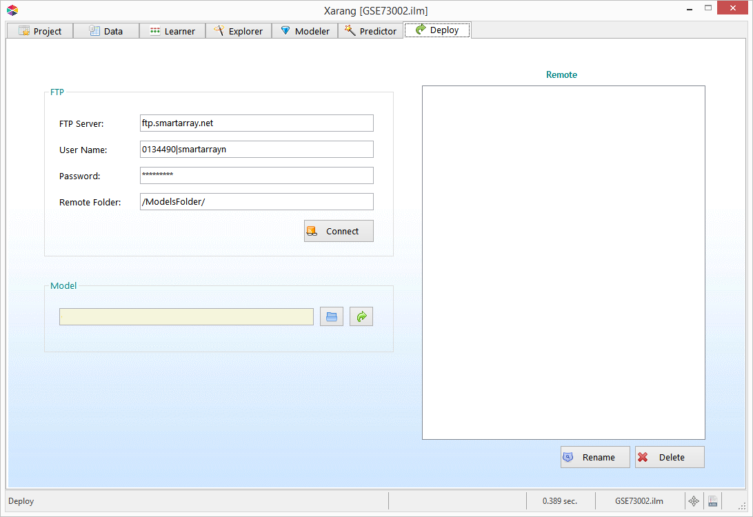
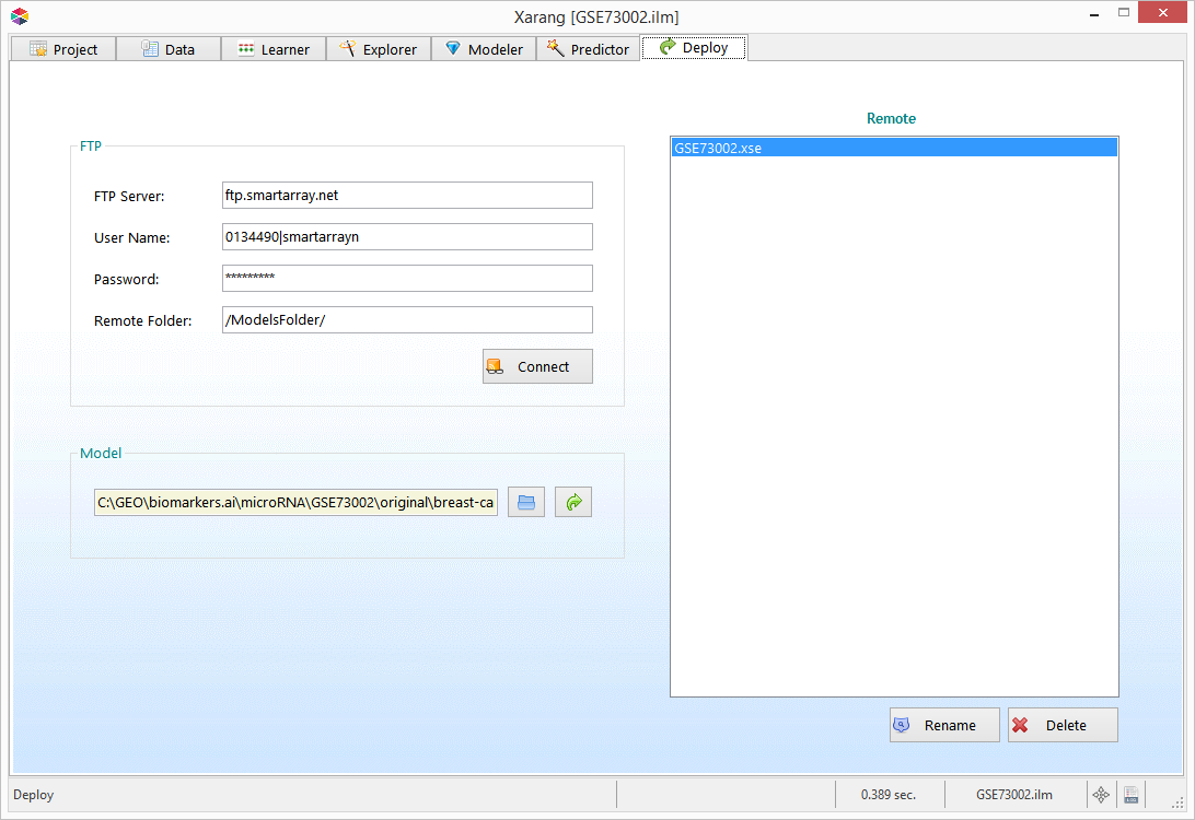
 to deploy the model to the remote server.
 .
. to predict using the model.
 or
or  to browse the current session queries.
 to refresh the list of models.
