| Map > Problem Definition > Data Preparation > Data Exploration > Modeling > Regression |
Modeling - Regression |
| I. Data Preparation |
|
1- Load libraries |
|
library(data.table) library(formattable) library(plotrix) library(limma) library(dplyr) library(Rtsne) library(MASS) library(xgboost) |
|
2- Read Expressions file |
|
df <- read.csv("GSE74763_rawlog_expr.csv") df2 <- df[,-1] rownames(df2) <- df[,1] expr <- transpose(df2) rownames(expr) <- colnames(df2) colnames(expr) <- rownames(df2) dim(expr) |
|
3- Read Samples file |
|
targets <- read.csv("GSE74763_rawlog_targets.csv") colnames(targets) dim(targets) |
|
4- Merge Expressions with Samples |
|
data <- cbind(expr, targets) colnames(data) dim(data) |
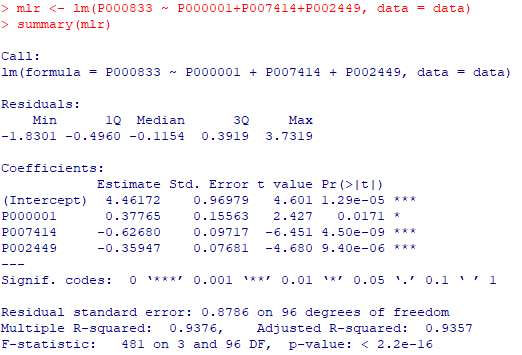
| II. MLR (Multiple Linear Regression) |
|
mlr <- lm(P000833 ~
P000001+P007414+P002449, data = data) summary(mlr) |
|
|
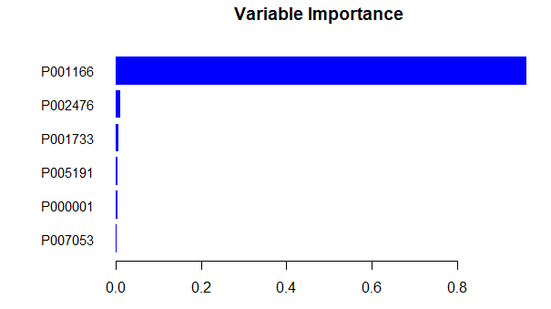
| III. XGBoost (Extreme Gradient Boosting) |
|
d1 <- data
|
|
|
| IV. Bioada SmartArray |
| Watch this video to learn how you can build regression models using Bioada Xarang significantly faster and easier. |