| Map
> Data Science > Predicting the Future >
Modeling >
Classification > Naive Bayesian |
|
|
|
|
|
|
Naive Bayesian
|
|
|
| The Naive Bayesian classifier is based on Bayes’ theorem with
the independence assumptions between predictors. A Naive Bayesian model is easy to build, with no complicated iterative
parameter estimation which makes it particularly useful for very large
datasets. Despite its simplicity, the Naive Bayesian classifier often does surprisingly well and is widely used because it often outperforms more sophisticated classification methods. |
|
|
|
|
|
|
|
Algorithm |
|
|
|
Bayes theorem provides a way of calculating the posterior probability,
P(c|x), from P(c),
P(x), and P(x|c).
Naive Bayes classifier assume that the effect of the value of a predictor (x)
on a given class (c) is independent of the values of other
predictors. This assumption is called class conditional independence. |
|
|
|

|
|
|
- P(c|x) is the posterior probability of
class (target) given predictor
(attribute).
- P(c) is the prior
probability of class.
- P(x|c) is
the likelihood which is the probability of predictor
given class.
- P(x) is the prior probability of
predictor.
|
|
|
| In ZeroR model there is no predictor, in OneR model
we try to find the single best predictor, naive Bayesian includes all
predictors using Bayes' rule and the independence assumptions between
predictors. |
|
|
| |
|
|
| Example 1: |
|
|
|
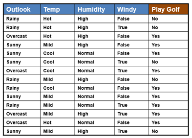
We use the same simple Weather dataset here. |
|
|
|
|
|
|
|
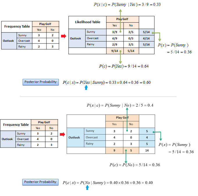
The posterior probability can be calculated by first,
constructing a frequency table for each
attribute against the target. Then, transforming the frequency tables to
likelihood tables and finally use the Naive Bayesian equation to calculate
the posterior probability for each class. The class with the highest
posterior probability is the outcome of prediction. |
|
|
|
|
|
|
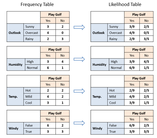
| The likelihood tables for all four predictors. |
|
|
|
|
|
|
| |
|
|
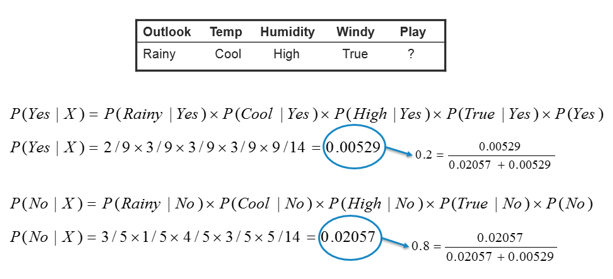
| Example 2: |
|
|
| In this example we have 4 inputs (predictors). The
final posterior probabilities can be standardized between 0 and 1. |
|
|
|
|
|
|
| |
|
|
| The zero-frequency problem |
|
|
| Add 1 to the count for every attribute value-class combination
(Laplace estimator) when an attribute value (Outlook=Overcast)
doesn’t occur with every class value (Play Golf=no). |
|
|
| |
|
|
| Numerical Predictors |
|
|
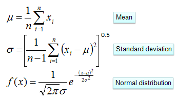
| Numerical variables need to be transformed to their
categorical counterparts (binning) before
constructing their frequency tables. The other option we have is using the
distribution of the numerical variable to have a good guess of the
frequency. For example, one common practice is to assume normal distributions for numerical
variables. |
|
|
| |
|
|
| The probability density function for the normal
distribution is defined by two parameters (mean and standard deviation). |
|
|
|
|
|
|
| |
|
|
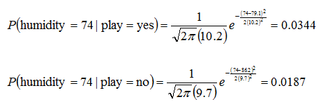
| Example: |
|
|
|
|
Humidity
|
|
Mean
|
StDev
|
| Play
Golf |
yes
|
86 |
96 |
80 |
65 |
70 |
80 |
70 |
90 |
75 |
79.1 |
10.2 |
|
no
|
85 |
90 |
70 |
95 |
91 |
|
|
|
|
86.2 |
9.7 |
|
|
|
| |
|
|
|
|
|
|
| |
|
|
| Predictors Contribution |
|
|
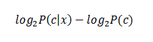
| Kononenko's information gain as a sum of information contributed by each
attribute can offer an explanation on how values of the predictors influence the
class probability. |
|
|
|
|
|
|
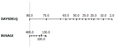
| The contribution of predictors can also be visualized
by plotting nomograms. Nomogram plots log odds ratios for each value of each
predictor. Lengths of the lines correspond to spans of odds ratios, suggesting importance of
the related predictor. It also shows impacts of individual values of the
predictor. |
|
|
|
|
|
|
| |
|
|
|
|
|
|
| |
|
|
 Try to invent a real time Bayesian classifier. You should be able to add
or remove data and variables (predictors and classes) on the fly.
Try to invent a real time Bayesian classifier. You should be able to add
or remove data and variables (predictors and classes) on the fly.
|
|
|
| |
|
|
|
|
|
|
|
|
|
