| Map > Problem Definition > Data Preparation > Data Exploration > Multivariate |
Data Exploration - Multivariate Analysis |
| I. Data Preparation |
|
1- Load libraries |
|
library(data.table) library(formattable) library(plotrix) library(limma) library(dplyr) library(Rtsne) |
|
2- Read Expressions file |
|
df <- read.csv("GSE74763_rawlog_expr.csv") df2 <- df[,-1] rownames(df2) <- df[,1] expr <- transpose(df2) rownames(expr) <- colnames(df2) colnames(expr) <- rownames(df2) dim(expr) |
|
3- Read Samples file |
|
targets <- read.csv("GSE74763_rawlog_targets.csv") colnames(targets) dim(targets) |
|
4- Merge Expressions with Samples |
|
data <- cbind(expr, targets) colnames(data) dim(data) |
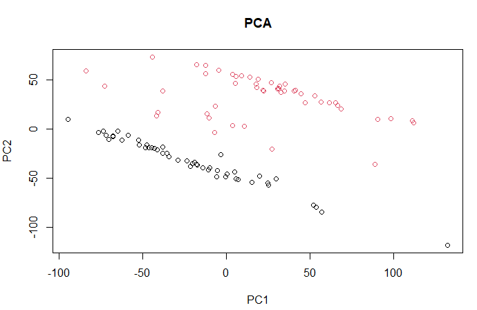
| II. PCA (Principal Components Analysis) |
|
d1 <- data d1$geo_accession <- NULL d1$gage <- NULL d1$gender <- NULL d1$target <- NULL pc <- prcomp(d1) groups <- as.fumeric(data$target) plot(pc$x[, 1], pc$x[, 2], main = "PCA", col=groups, xlab = "PC1", ylab = "PC2") |
|
|
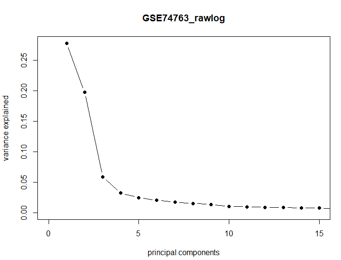
| This PCA is equivalent to performing the SVD on the centered data, where the centering occurs on the columns (here probes). |
|
cx <- sweep(d1, 2, colMeans(d1), "-") sv <- svd(cx) names(sv) plot(sv$d^2/sum(sv$d^2), xlim = c(0, 15), type = "b", pch = 16, xlab = "principal components", ylab = "variance explained", main="GSE74763_rawlog") |
|
|
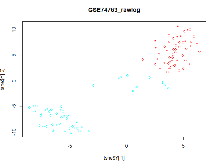
| III. t-SNE (t-distributed Stochastic Neighbour Embedding) |
| d1 <- data d1$geo_accession <- NULL d1$gage <- NULL d1$gender <- NULL d1$target <- NULL groups <- as.fumeric(data$target) colors =
rainbow(length(unique(groups))) |
|
|
| IV. Bioada SmartArray |
| Watch this video to learn how you can perform multivariate analysis using Bioada SmartArray significantly faster and easier. |