| Map > Problem Definition > Data Preparation > Data Exploration > Modeling > Evaluation > Regression |
Evaluation - Regression |
| I. Data Preparation |
|
1- Load libraries |
|
library(data.table) library(formattable) library(plotrix) library(limma) library(dplyr) library(Rtsne) library(MASS) library(xgboost) |
|
2- Read Expressions file |
|
df <- read.csv("GSE74763_rawlog_expr.csv") df2 <- df[,-1] rownames(df2) <- df[,1] expr <- transpose(df2) rownames(expr) <- colnames(df2) colnames(expr) <- rownames(df2) dim(expr) |
|
3- Read Samples file |
|
targets <- read.csv("GSE74763_rawlog_targets.csv") colnames(targets) dim(targets) |
|
4- Merge Expressions with Samples |
|
data <- cbind(expr, targets) colnames(data) dim(data) |
| II. Splitting Data into Training and Test Sets |
|
set.seed(101) sample = sample.split(data$P000833, SplitRatio = .8) train = subset(d1, sample == TRUE) test = subset(d1, sample == FALSE) dim(train) dim(test) |
| II. MLR Model |
|
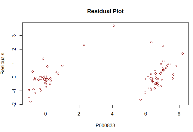
mlr <- lm(P000833 ~
P000001+P007414+P002449, data = train) summary(mlr) #Residual
plot |
|
|
|
#Q-Q plot stdres = rstandard(mlr) qqnorm(stdres, ylab="Standardized Residuals", xlab="Normal Scores", main="QQ Plot") qqline(stdres) |
|
|
|
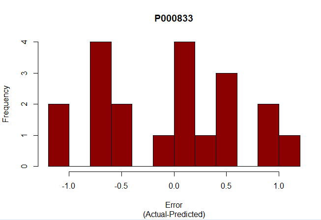
#Test pred <- predict(mlr, newdata=test) errors <- test$P000833 - pred rmse <- sqrt(mean((errors^2))) print(rmse) #Erros histogram hist(errors, main="P000833", sub="(Actual-Predicted)", xlab="Error", breaks=10, col="darkred") |
|
|
|
|
| IV. Bioada Xarang |
| Watch this video to learn how you can build, test and deploy regression models using Bioada Xarang significantly faster and easier. |