| Map > Problem Definition > Data Preparation > Data Exploration > Modeling > Clustering |
Modeling - Clustering |
| I. Data Preparation |
|
1- Load libraries |
|
library(data.table) library(formattable) library(plotrix) library(limma) library(dplyr) library(Rtsne) library(MASS) library(xgboost) library(factoextra) |
|
2- Read Expressions file |
|
df <- read.csv("GSE74763_rawlog_expr.csv") df2 <- df[,-1] rownames(df2) <- df[,1] expr <- transpose(df2) rownames(expr) <- colnames(df2) colnames(expr) <- rownames(df2) dim(expr) |
|
3- Read Samples file |
|
targets <- read.csv("GSE74763_rawlog_targets.csv") colnames(targets) dim(targets) |
|
4- Merge Expressions with Samples |
|
data <- cbind(expr, targets) colnames(data) dim(data) |
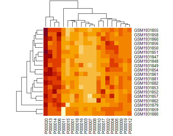
| II. Heatmap |
| heatmap(as.matrix(expr[1:20, 1:20])) |
|
|
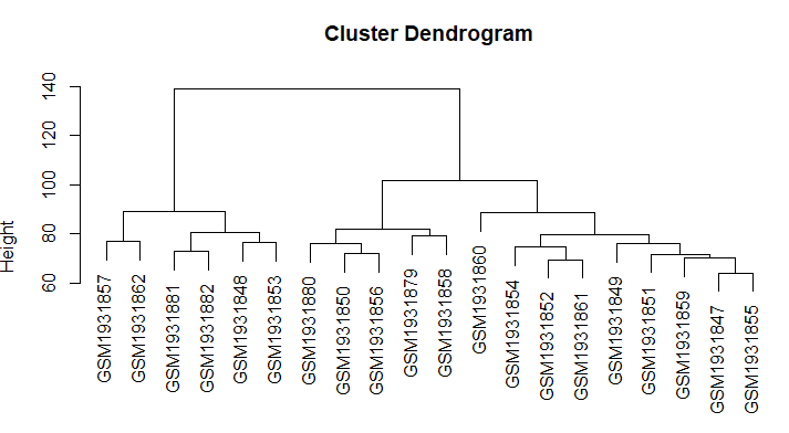
| II. Hierarchical Clustering |
|
# Dissimilarity matrix d <- dist(expr[1:20, 1:400], method = "euclidean") # Hierarchical clustering using Complete Linkage hc1 <- hclust(d, method = "complete" ) # Plot the obtained dendrogram plot(hc1, cex = 1, hang = 0.1) |
|
|
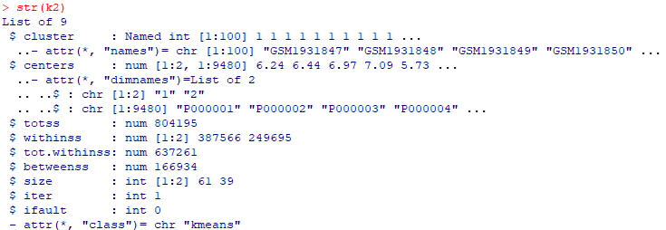
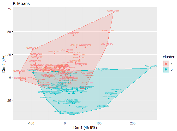
| III. K-Means Clustering |
|
k2 <- kmeans(expr, centers = 2,
nstart = 25) |
|
|
|
|
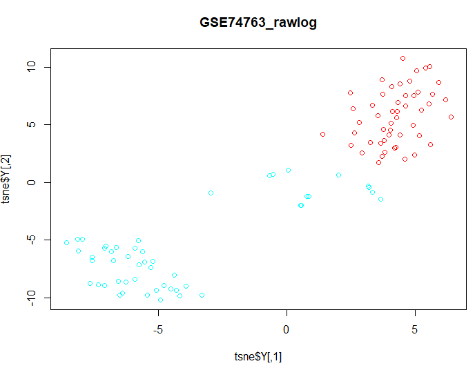
| IV. t-SNE (t-distributed Stochastic Neighbour Embedding) |
| d1 <- data d1$geo_accession <- NULL d1$gage <- NULL d1$gender <- NULL d1$target <- NULL groups <- as.fumeric(data$target) colors =
rainbow(length(unique(groups))) |
|
|
| V. Bioada SmartArray |
| Watch this video to learn how you can build clustering models using Bioada SmartArray significantly faster and easier. Bioada only supports t-SNE. |