| Map > Problem Definition > Data Preparation > Data Exploration > Modeling > Classification |
Modeling - Classification |
| I. Data Preparation |
|
1- Load libraries |
|
library(data.table) library(formattable) library(plotrix) library(limma) library(dplyr) library(Rtsne) library(MASS) library(xgboost) |
|
2- Read Expressions file |
|
df <- read.csv("GSE74763_rawlog_expr.csv") df2 <- df[,-1] rownames(df2) <- df[,1] expr <- transpose(df2) rownames(expr) <- colnames(df2) colnames(expr) <- rownames(df2) dim(expr) |
|
3- Read Samples file |
|
targets <- read.csv("GSE74763_rawlog_targets.csv") colnames(targets) dim(targets) |
|
4- Merge Expressions with Samples |
|
data <- cbind(expr, targets) colnames(data) dim(data) |
| II. Variable Selection |
| Here, we use t-test to select the topN variables (probes) from 9480 probes. |
|
d1 <- data groups <- as.fumeric(data$target) tval <- lapply(d1, function(x) { t.test(x ~ groups)$statistic }) tdf <- as.data.frame(t(as.data.frame(tval))) colnames(tdf) tdf$t <- abs(tdf$t) tdfo <- tdf[order(tdf$t,decreasing=TRUE),,drop=FALSE] head(tdfo) |
|
|
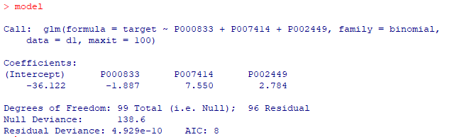
| III. Logistic Regression |
|
d1 <- data d1$geo_accession <- NULL d1$age <- NULL d1$gender <- NULL d1$target <- as.fumeric(d1$target)-1 model <- glm(target ~ P000833+P007414+P002449, data = d1, family = binomial, maxit = 100) print(model) |
|
|
| IV. XGBoost (Extreme Gradient Boosting) |
| XGBoost does not need a variable selection step. |
| d1 <- data d1$geo_accession <- NULL d1$age <- NULL d1$gender <- NULL d1$target <- as.fumeric(d1$target)-1 |
|
|
| V. Bioada SmartArray |
| Watch this video to learn how you can build classification models using Bioada SmartArray significantly faster and easier. |