Introduction Last updated: 2020-07-31

There are many factors that make data preparation challenging, from understanding where to find the data to extracting it, then properly formatting it and finally loading it to a database management system (DBMS). SmartArray reduces data preparation time, so that you the focus is on using a high quality and enriched data for visualization, statistical analysis and predictive modeling. With Bioada, users have the full control on the data.

SmartArray provides a unique interactive data exploration platform for ad-hoc queries, data visualizations and statistical analysis. Users can explore data interactively and apply statistical models and analytical techniques to find potential biomarkers in the genomic data.Users can focus and emphasize on interactivity and effective integration of techniques from data science.

Genomic datasets are high-dimensional molecular profiles pose challenges to data interpretation and hypothesis generation. SmartArray has a method that discovers significantly enriched pathways and gene ontology terms across datasets. SmartArray enrichment is a versatile method that improves systems-level understanding of cellular entities in health and disease through integration of genomic datasets and pathway and gene ontology annotations
Home

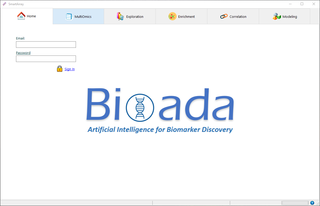
The Home tab is the first screen of SmartArray. Every user is given a set of credentials to login to the application according to their roles.

Login

  1. Enter Email and password in the related fields
  2. Click on to SignIn

Add User

Admins have access to add/edit/delete users

  1. Sign-in to the application
  2. Click on "User" icon.A message box appears as below.
  3. Enter the new email, password, and confirm password in the related fields.
  4. Once the user is saved the below popup appears

Edit User

This feature activates, inactivates, or deletes a user.

Activate User:

  1. Sign-in to the application
  2. Click on "User" icon.
  3. Click on the button.All the Inactive users will be displayed under "Inactive Users" list .
  4. Select an user to Activate and click on the Active button.A confirmation message appears as shown below.
  5. Once the user is activated, it will be displayed under active users list.

Inactivate User:

  1. Sign-in to the application
  2. Click on "User" icon.
  3. Click on the button.All the active users will be displayed under "Active Users" list.
  4. Select an user to inactivate and click on the Inactivate User button.A confirmation message appears as shown below.
  5. Once the user is inactived, it will be displayed under inactive users list.

Delete User:

  1. Sign-in to the application
  2. Click on "User" icon.
  3. Click on the button.All the active users will be displayed under "Active Users" and inactive users on "Inactive Users" related lists .
  4. Select an user to delete and click on the Delete User button.A confirmation message appears as shown below.On click of "Ok" the user will be deleted permanently.

Data

The Data(GSE) tab allows you to load data from database,add new data to database and compare two different databases.

Load

Loads all the existing databases

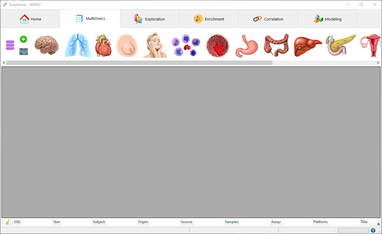
  1. Click on button.It loads the existing databases in the local database server.
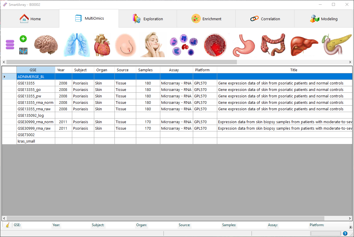
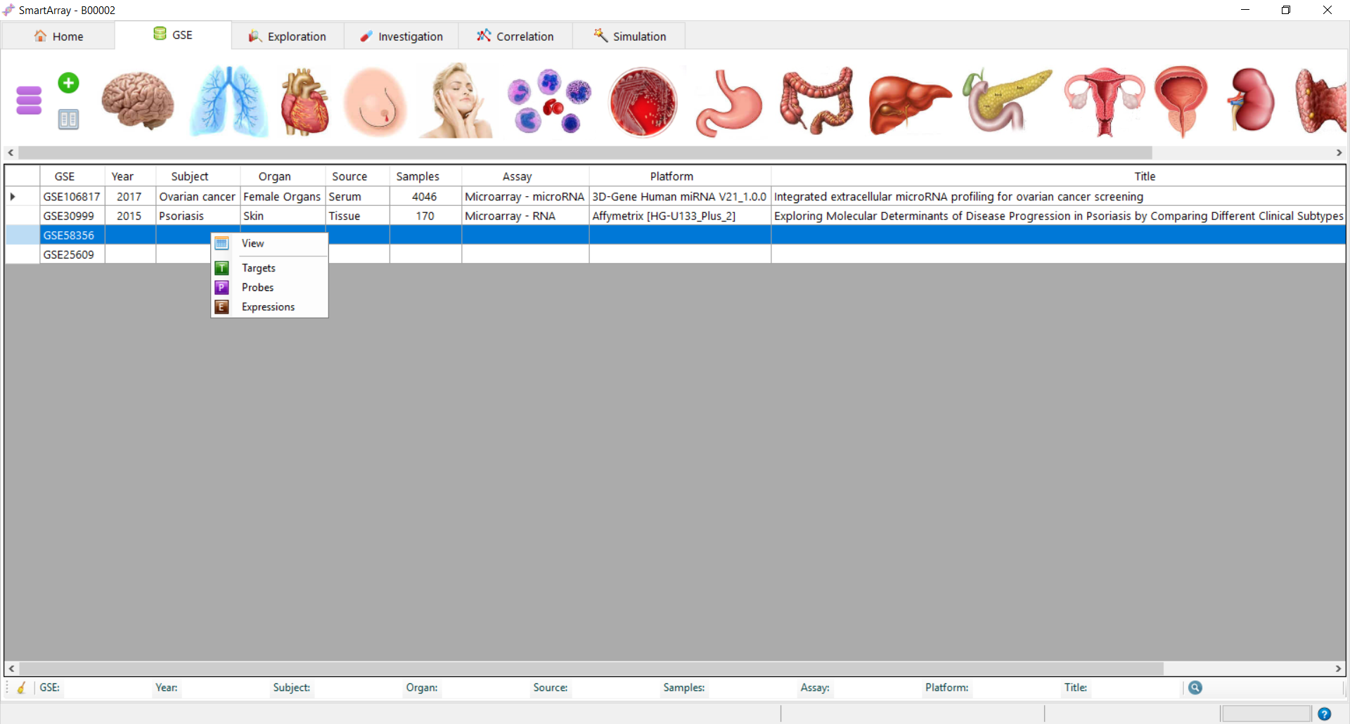
  2. The multiple filters(GSE, Year, Subject, Organ, Source, Samples, Assay, Platform, Title) at the bottom of the screen can be used to filter the databases
  3. Right click on any GSE to view the details.
  4. Enter the details of the dataset and click on Apply/OK.
  5. Delete GSE button can be used to delete the GSE from the database server.
  6. Right click on Targets to get the target file details.
  7. Click on to run the query and the results are as shown above.
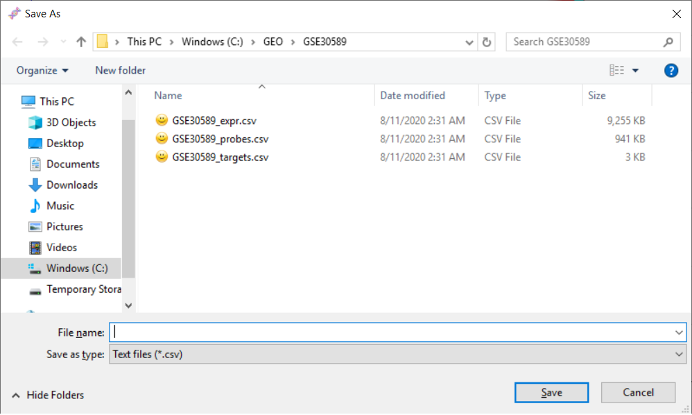
  8. Click on to save the query results.
  9. Click on to get the aggreagte of the selected column.
  10. Similar results are obtained for Probes and Expressions.

New

Adds a new database to the local database server

  1. Click on button.A new window is opened as shown below.
  2. Click on . Enter new database name and click OK.
  3. The newly added database appears in the GSE list. Select the database and click on to connect
  4. Click on the Expressions hyperlink and select the expression file to be uploaded.
  5. The probes and target files are automatically uploaded on selection of expression file.
  6. Click on various Check buttons to ensure all the files are intact.
  7. Go to Targets tab and click on to upload the data to database.Click on to view the file.
  8. Go to Probes tab and click on to upload the data to database.Click on to view the file.
  9. Go to Expressions tab and click on to upload the data to database.Click on to view the file.
  10. Go to Enrichment tab and click on Expression File hyperlink to select the expression file to transform the data.
  11. Select on the Probe/Gene depending on the data.
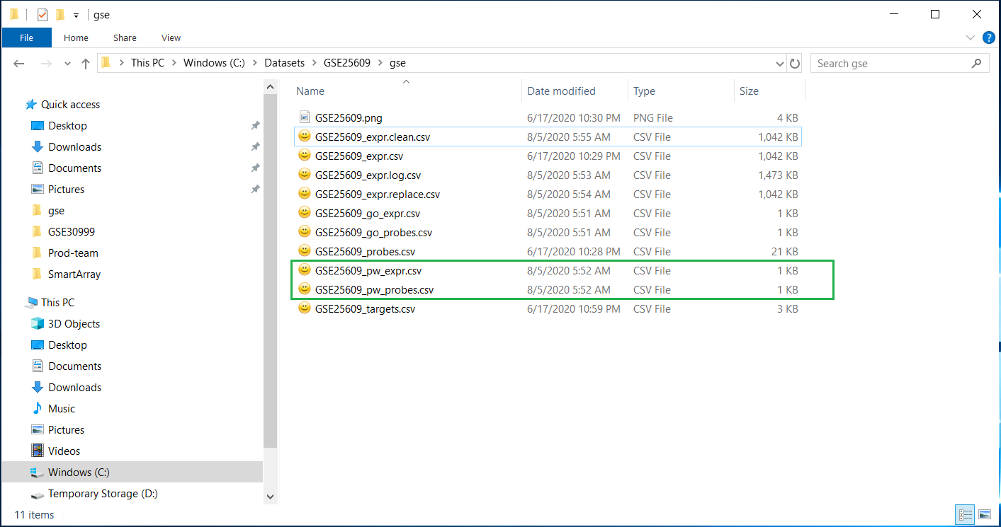
  12. Click on Reactome Pathway button to compress the data to higher pathway.This creates a new pathway file with Probe and Sample details.
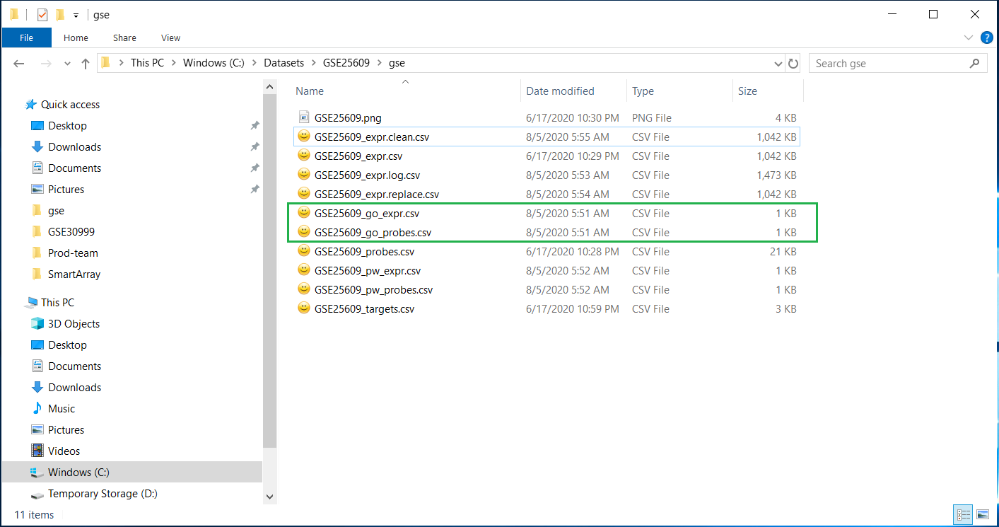
  13. Click on Gene Ontology button.
  14. Click on for Log transformation. This transforms the expression file to log expression and saves the file.Below is sample of log expression file.
  15. Click on to replace any missing value with the average value of corresponding row. This modifies the expression file and saves the file.Below is sample of replaced file.
  16. Click on to delete any empty row . This changes the expression file and saves the file.Below is sample of clean file.

Compare

Compare two databases of same category

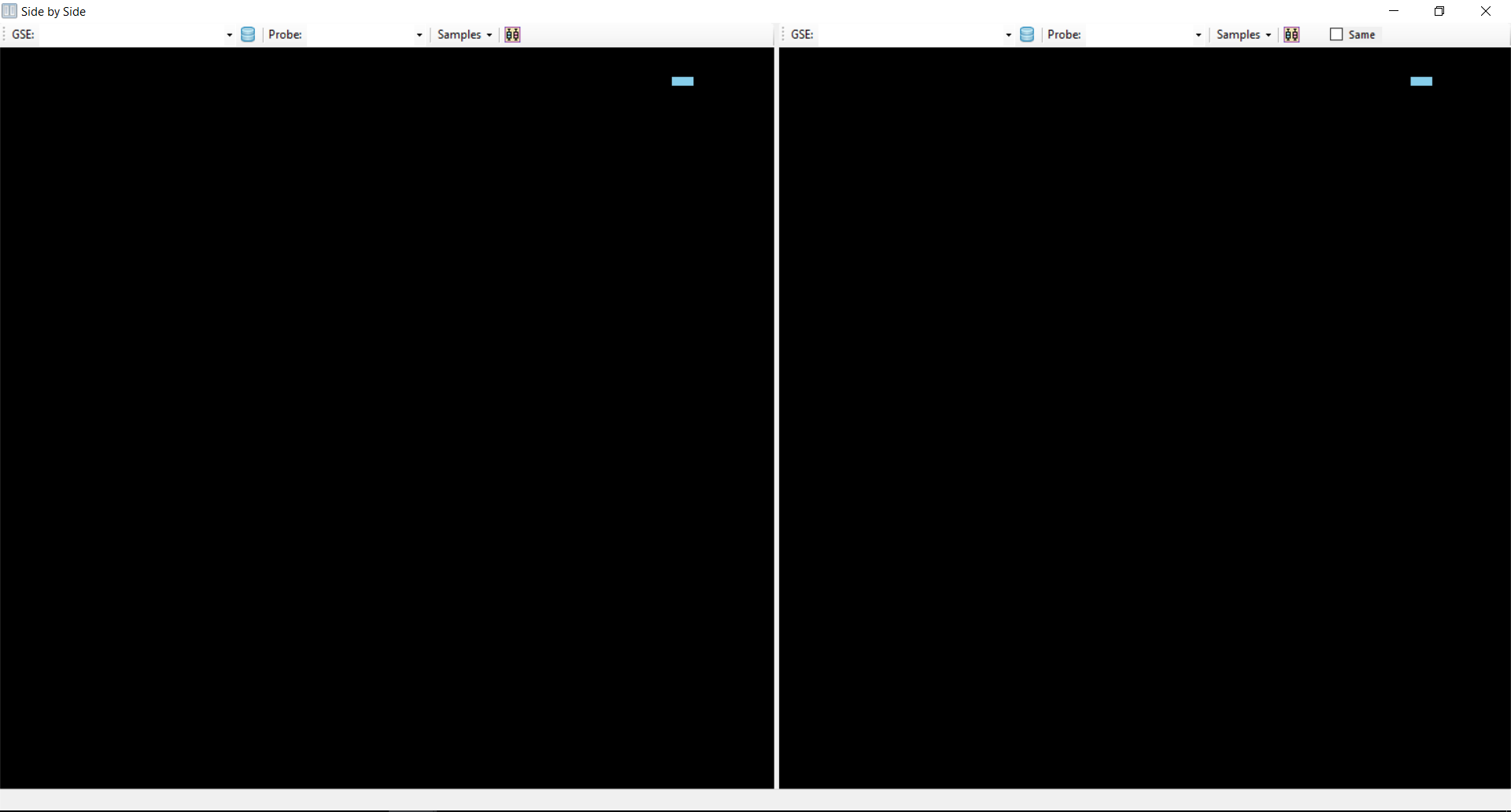
  1. Click on .A new compare window opens up.
  2. Select two databases that similar to same category for comparison
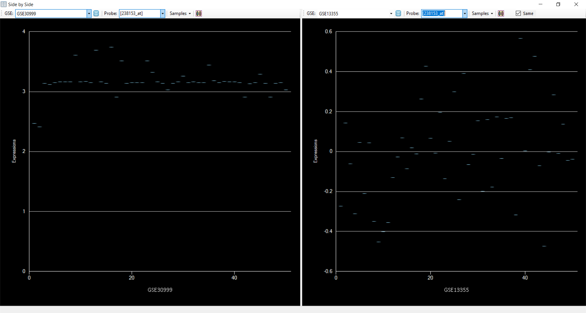
  3. Click on to get the distribution of data from both datasets
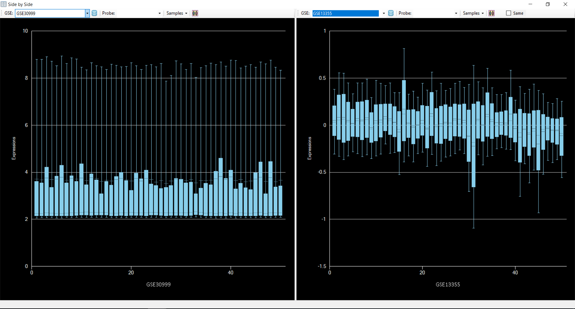
  4. Click on Same checkbox to compare the same samples on either sides if available
  5. Select probes on each side to compare individual probes in the datasets.
  6. Click on Samples dropdown for filters.Click on Add Filter
  7. Select the filters to apply and the filtered data will be displayed under GSM Samples on click.
  8. Click on Refresh link to clear all the filters or click on "OK" to apply the filter.
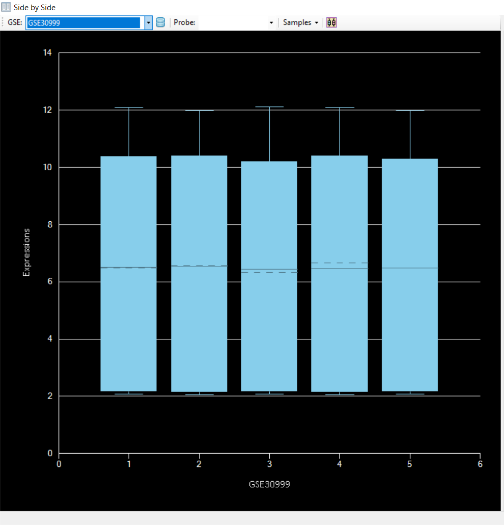
  9. Click on View Filter to check the filters applied.
  10. Click on Delete Filter to delete the existing filter.
Exploration

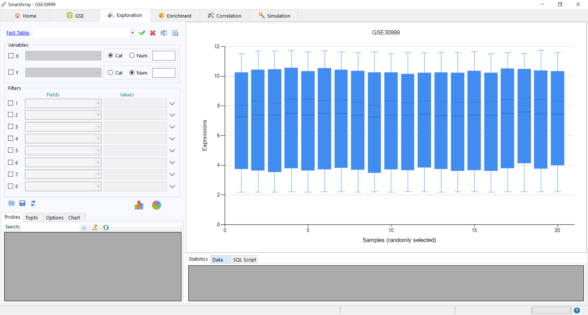
The exploration tab performs the statistical analysis on the database.Upon double clicking on the database in GSE tab, it redirects to the default page of Exploration tab.

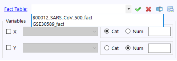
  1. Click on the Fact Table hyperlink to load the fact tables from the database.Select the corresponding fact table and click on to load the table. The original fact table cannot be deleted,renamed or exported.
  2. Click on to delete the fact table.
  3. Click on to rename the fact table.
  4. Click on to export the fact table.

Univariate

Univariate analysis on a numerical or categorical variant can be performed.

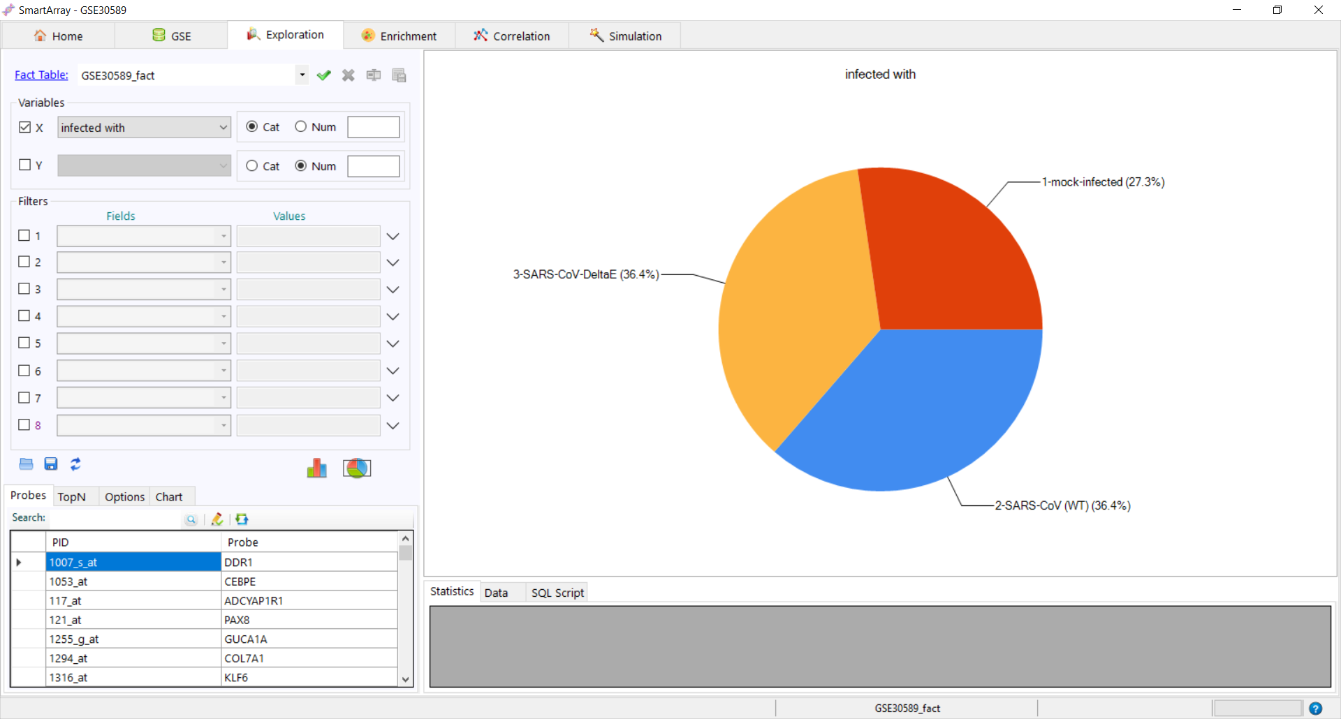
  1. Select any variant as X variable to perform univariate analysis.Depending on the variant selected, the type is changed to Cat(Categorical) or Num(Numerical)
  2. Click on to get the distribution of the variant. The data and the SQL Script used can be seen at the bottom of the screen.
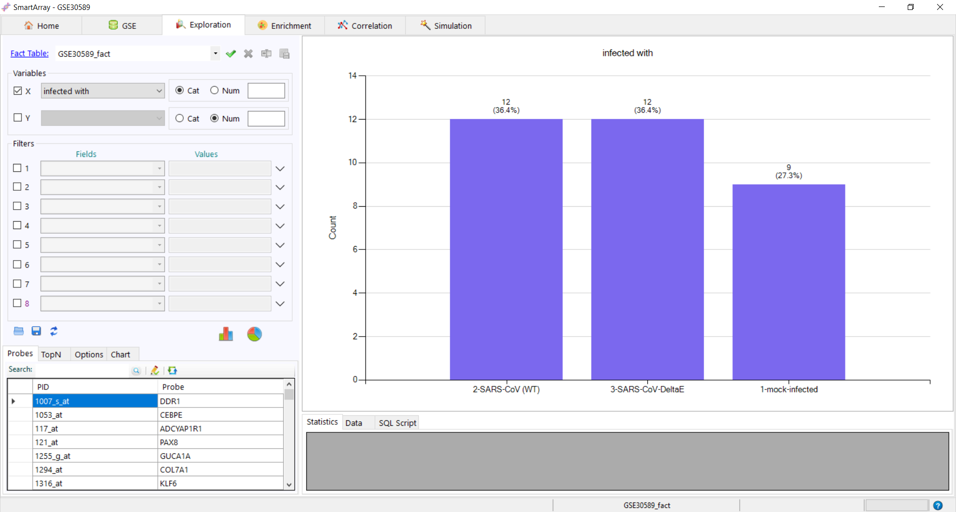
  3. Click on to get the pie chart distribution.
Bivariate

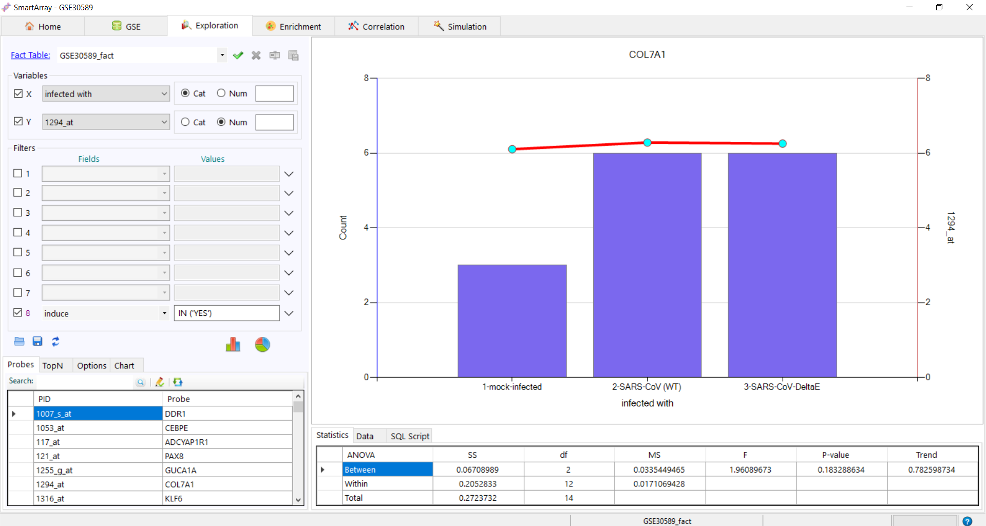
Bivariate analysis on a numerical or categorical variant can be performed.

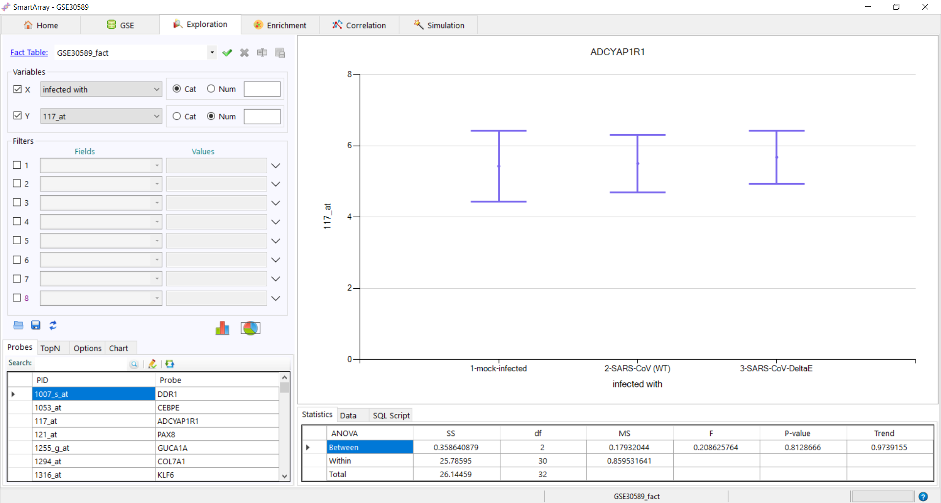
  1. Select any variant as Y variable to perform bivariate analysis.Depending on the variant selected, the type is changed to Cat(Categorical) or Num(Numerical)
  2. Click on to get the distribution of the variant. The statistics, data and the SQL Script used can be seen at the bottom of the screen.
  3. Click on to get the pie chart distribution.
  4. Keep changing the values in the Y variable to get the correlation of each value with X variant.

Visualization

The top 5,100 or 800 subsets can be sliced to form another dataset.

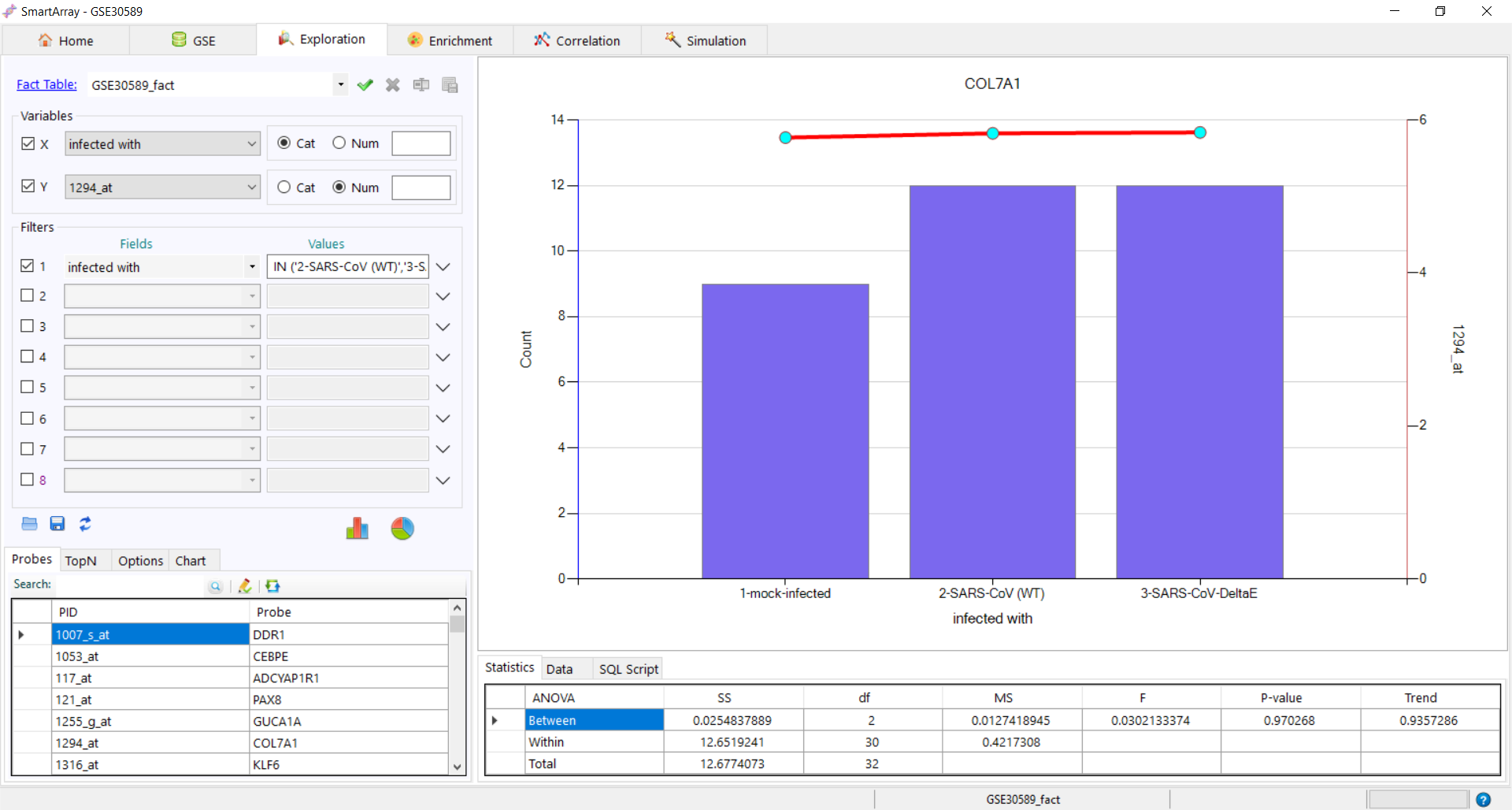
  1. Filters: Apply filters for more clear view of the data.7 Filters (Filter 1- 8) can be applied for filter functionality.
    • Select a variable to apply the filter.Click on or to see the result.
    • Filter No. 8 adds another dimension to the data.Click on or to see the result.
    • Click on to refresh the existing filters.
    • Click on to save the data.
    • Click on to load the saved filters.
  2. Probes: The correlation between each value of Y variable with any X variant can be seen in the Probes Tab.
    • Keep clicking on different values to see the distribution changing in box plot.
    • Enter the probe ID/name to search and click on to search the next matching value.
    • Select the probe to be renamed and click on to rename the probe.
    • Click on to refresh the data.
  3. Top: Allows users to see the correlation between all the values in Y variable with respect to X variable.
    • Click on All dropdown to filter the data to be displayed.
      1. All - Displays the complete data
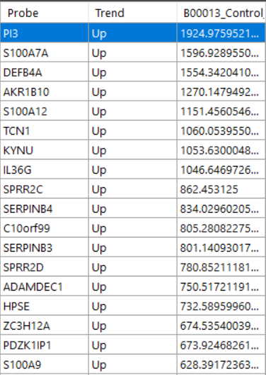
      2. Upregulated - Displays the data that has trend Up
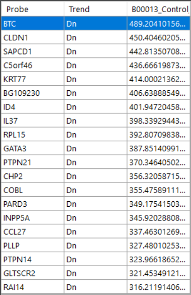
      3. Downregulated - Displays the data that has trend Down(Dn)
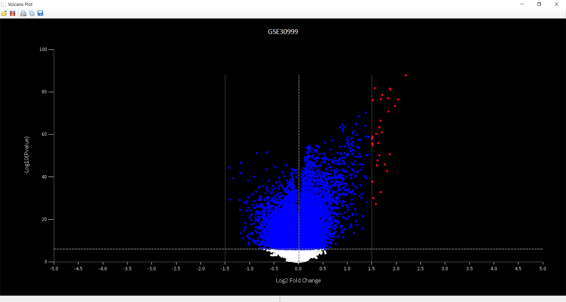
    • Click on to get the Volcano/Manhattan plot.

      Click on to load the data used for obtaining volcano plot.

      Click on to save the data used for obtaining volcano plot.

      Click on to print the volcano plot.

      Click on to copy the volcano plot.

      Click on to save the volcano plot.

    • Click on to search for Probe ID or Probe name.
    • Click on to save the top N data where N can be in the range of 5 to 800.
    • Click on to load the existing subset dataset.
    • Click on to save the Top N data to database.The textbox can be used to name the table and the number of rows(N) to be saved. The saved dataset appears on the Fact_Table list
  4. Options tab provides more features for SNPs.
    • Exclude NC (No Call): Excludes NC genotype for the statistical analysis
    • Encode SNP: Encodes the SNPs
    • In-memory Aggregation: This feature allows users to use the in-memory of their local computers to run SmartArray application
  5. Chart tab provides more features on visualization.
    • Font Size: Increasing or decreasing of font size changes the font displayed on the charts
    • Click on Density Plot to get the density plot for the dataset.
    • To copy the density plot, use and edit it in any image editor.
    • Click on to print the density plot.
    • Click on to save the density plot.
    • X-axis Show Range: Shows the range of values in X-axis.
    • Y2 % Format: Shows the plot with y-axis values in terms of percentage.
    • Volcano Plot: Check on this item to show the volcano plot after running. Uncheck to not show the plot. CLick on to show the saved plot
    • X-axis Sort by Count: Sorts the data according to the x-axis value count.
    • Minimum Y-Axis: Use minimum value of Y-axis instead of 0 as minimum value.
    • Log2FC: It takes the value of (Log2(B)- Log2(A)) if checked and B - A if unchecked in X-axis of the volcano plot.
    • X-axis Reversed: Reverses the X-axis and displays the plot.
    • -Log10(Pvalue): On check considers -Log10(Pvalue) as Y-axis value else takes the score as Y-value in the volcano plot.

Enrichment

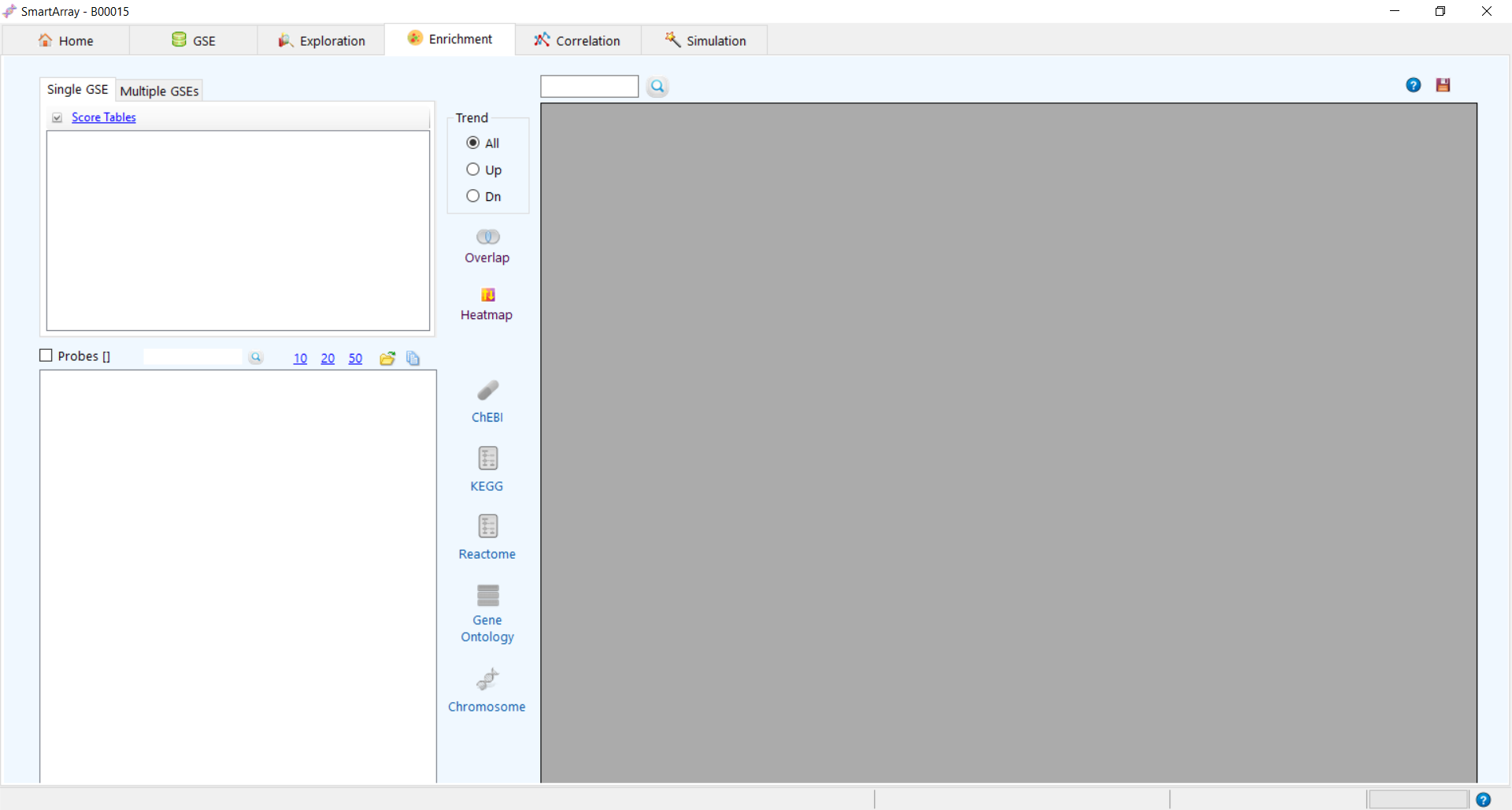
Enrichment displays the relation of probes with chemicals, pathways, gene ontology and chromosomes. The chemical details are saved in the database.

Click on Score Tables to load the subset datasets.

  1. Click on Overlap to see the probes.
  2. Click on Heatmap to see the heatmap of all probes
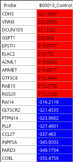
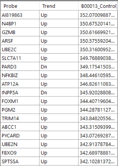
  3. Trend Options allows to see the trend of probes.
    • All - Displays all the probes of subset.
    • Up - Displays probes that are up regulated.
    • Down - Displays probes that are down regulated.
  4. Textbox can be used to search for probes.

Chemical Interaction

Multiple chemical interactions can be seen in Enrichment tab. Click on numbers or the checkbox to select the probes.

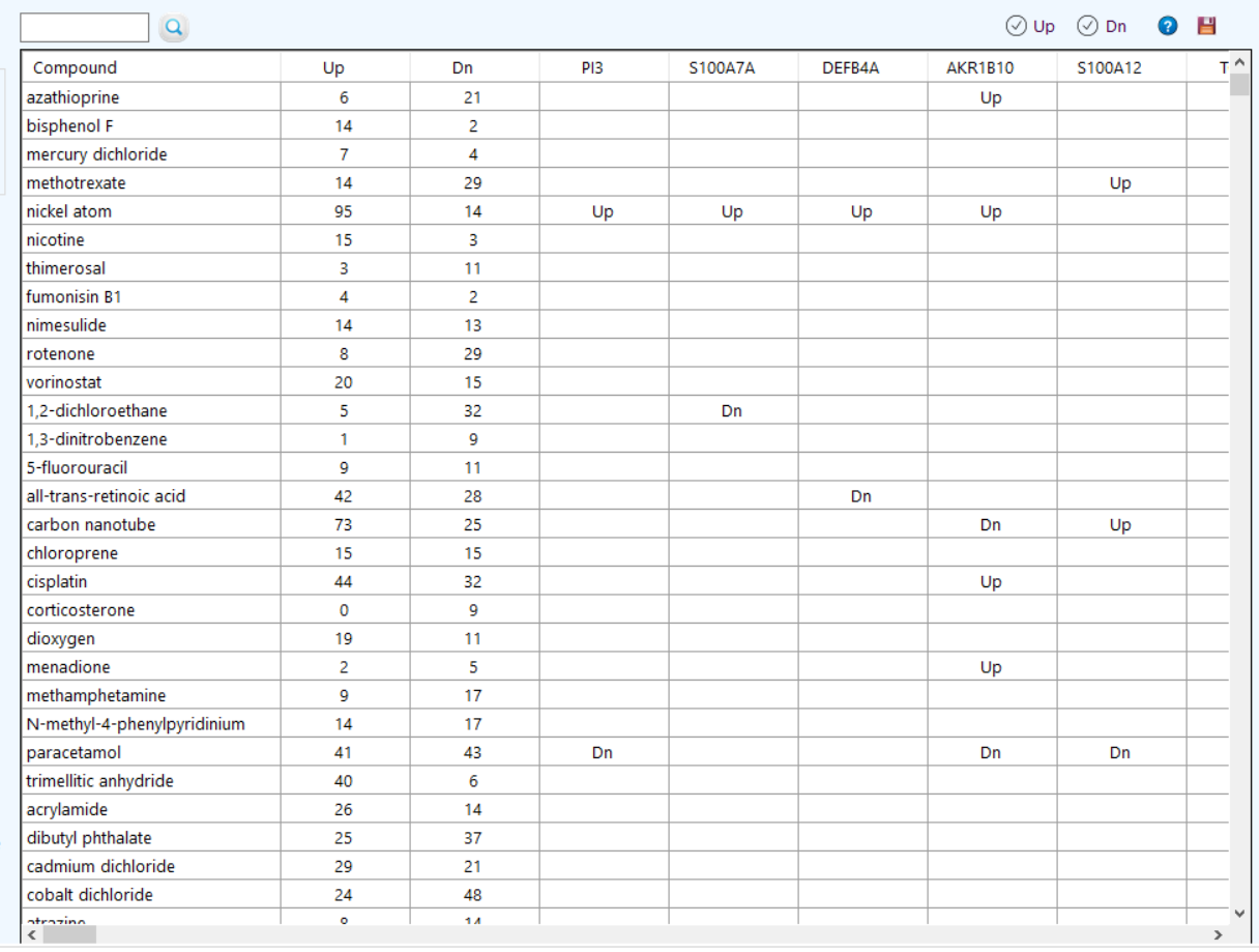
  1. Click on ChEBI to see the Gene-Compound interactions in probes.
    • Click on Up to see the up regulated probes.
    • Click on Dn to see the down regulated probes.
    • Click on to see the ChEBI qualifiers.
    • Click on to save the results.
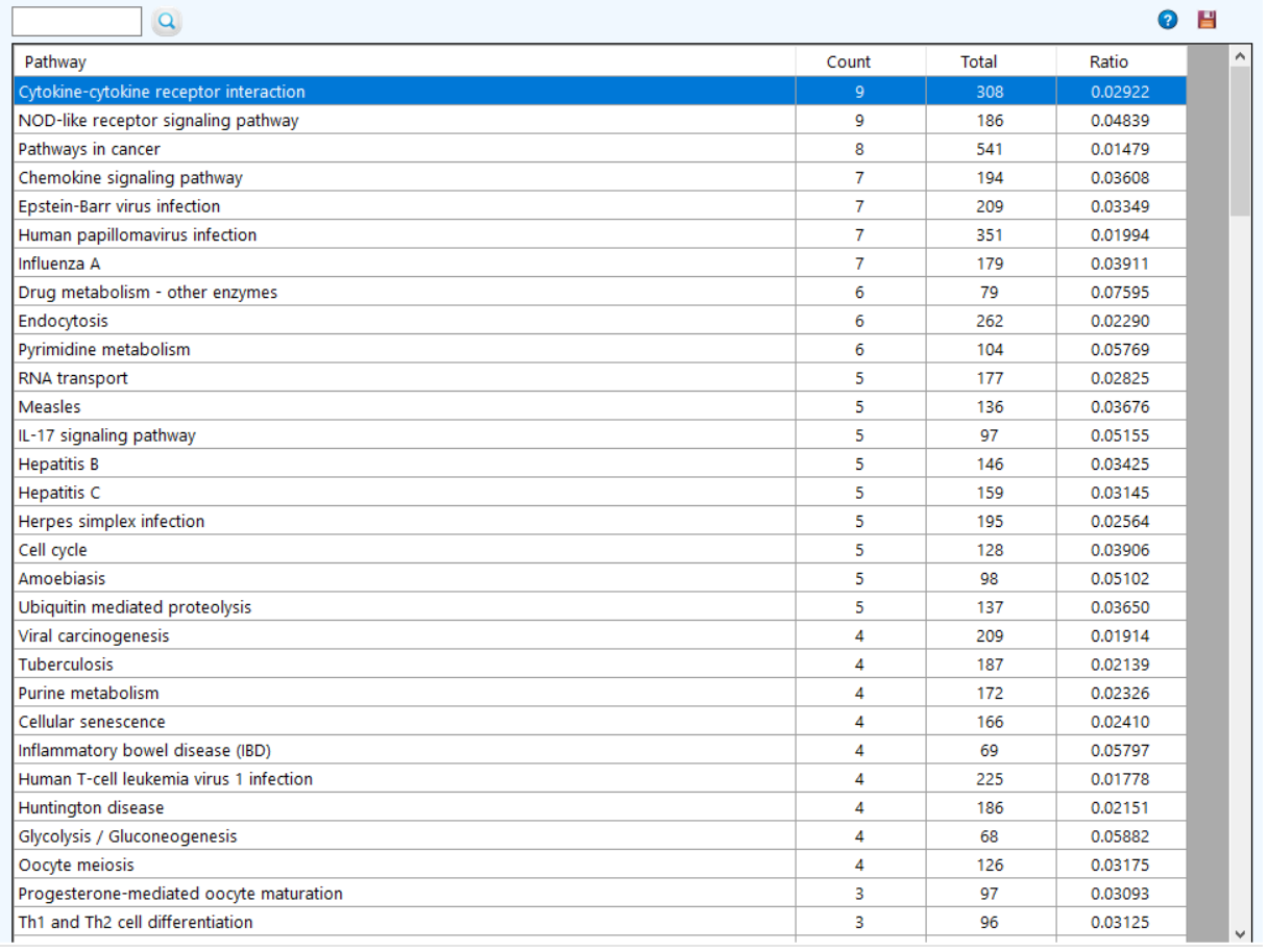
  2. Click on to see the KEGG pathway enrichment.
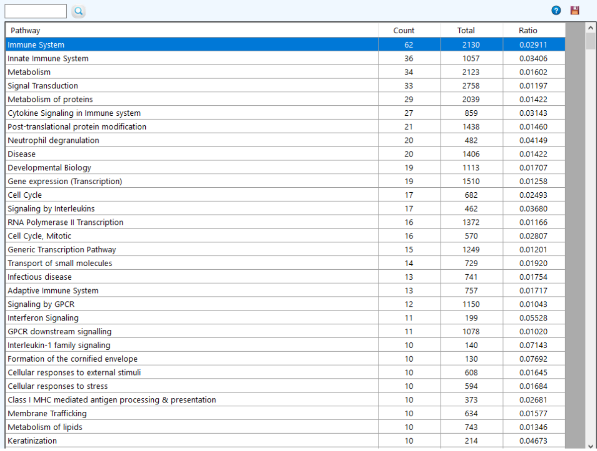
  3. Click on to see the reactome pathway enrichment.
  4. Click on to see the gene ontology pathway enrichment.
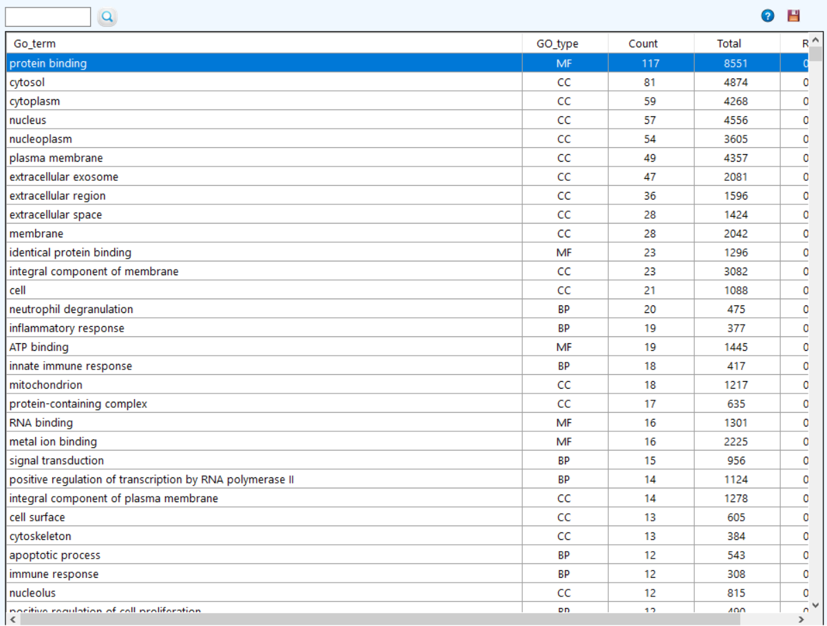
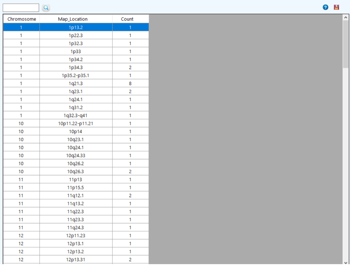
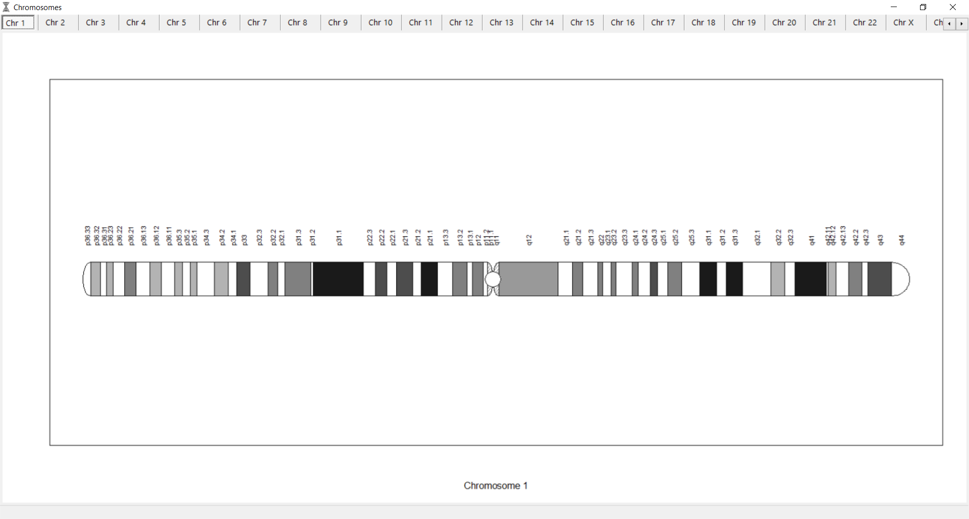
  5. Click on to see the chromosomes frequency.
  6. Click on Map hyperlink to see the chromosome map.

Correlation

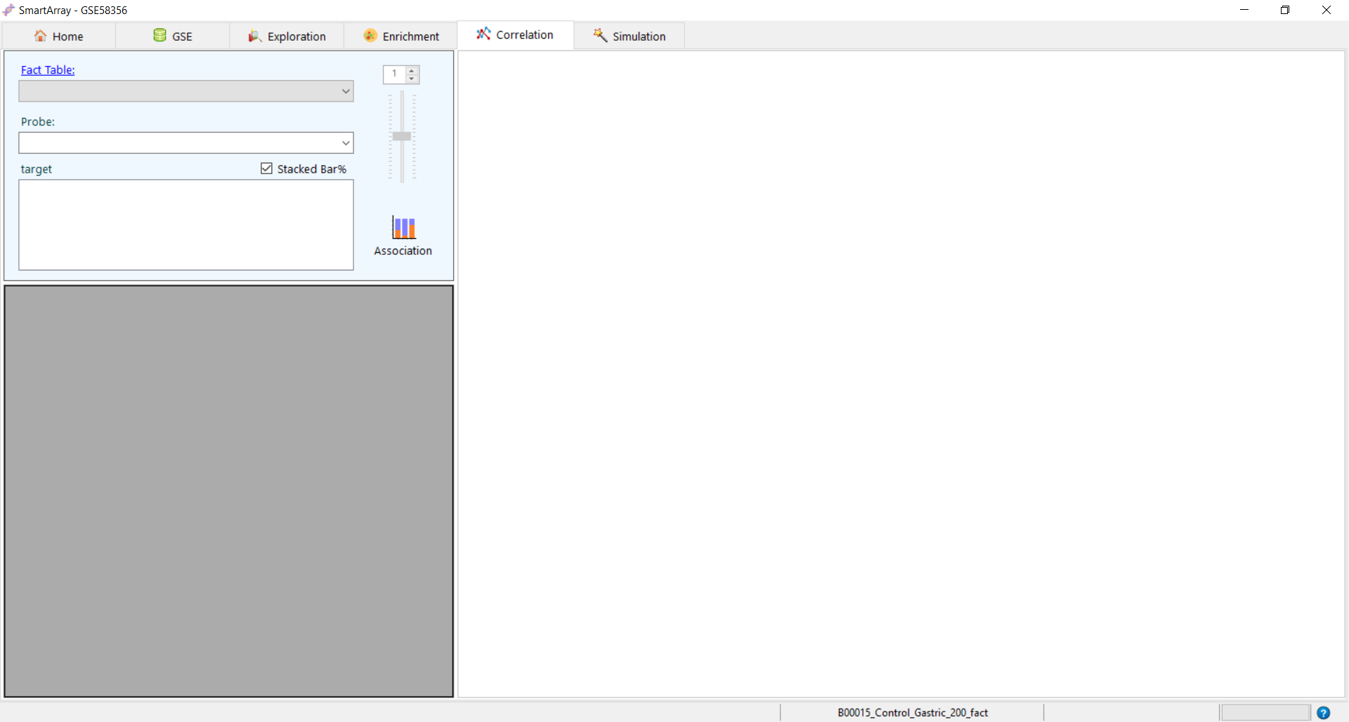
This tab gives the correlation between probes in a dataset.Correlation can be observed only for smaller datasets which are manually saved.

  1. Click on Fact Table hyperlink to load the saved datasets.
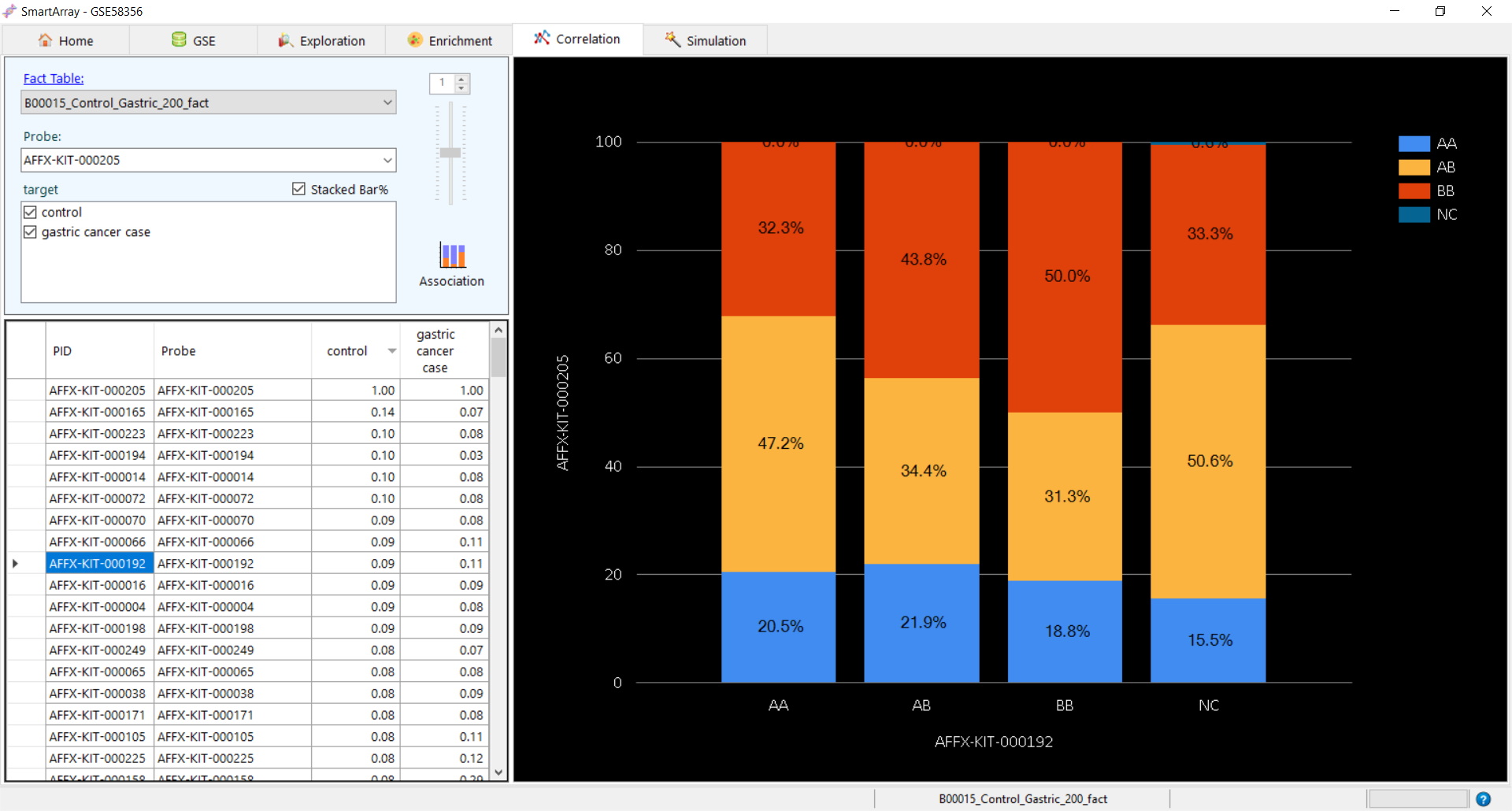
  2. Select a probe/SNP and click on - Correlation in case of probes or Association in case of SNPs
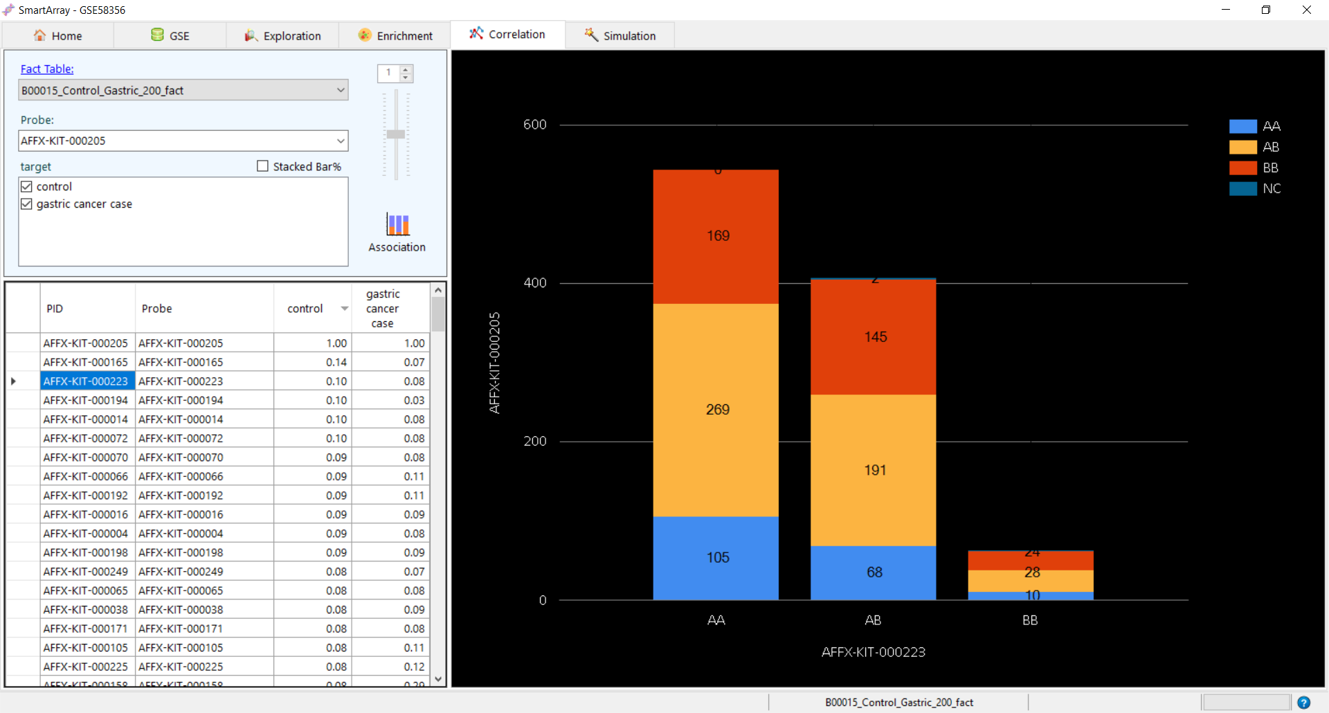
  3. Unchecking of Stacked Bar% gives the plot with the count of SNPs instead of percent.
  4. The zoom option is enabled for probes and can be used to change the offset of Y-axis.

Simulation

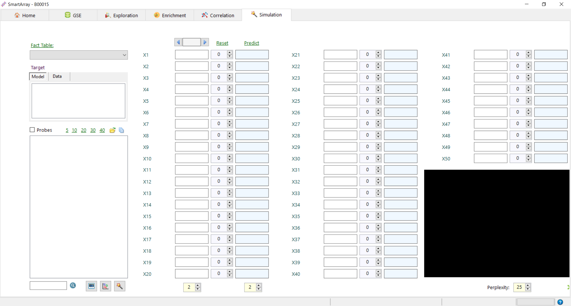
Simulation tab extends the correlation feature and renders the simulation based on the target and data.

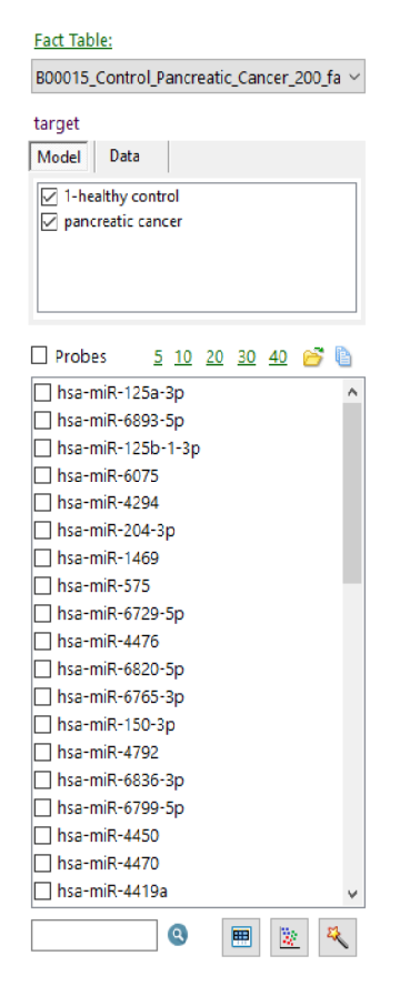
Click on the Fact_Table hyperlink to load the subsets.

Build Models

The simulation models can be generated by using various target and data combinations.

  1. Select the target and the data that should be tested with the model.
  2. Select the number of probes for which the model should be generated.All the probes can be selected by checking the checkbox or the Top N probes can be selected by clicking on the available number hyperlinks
  3. Click on to load any external probes.
  4. Click on to copy the probes list.
  5. Search text box can be used to search for any probe in the list
  6. Click on to build simulation models.
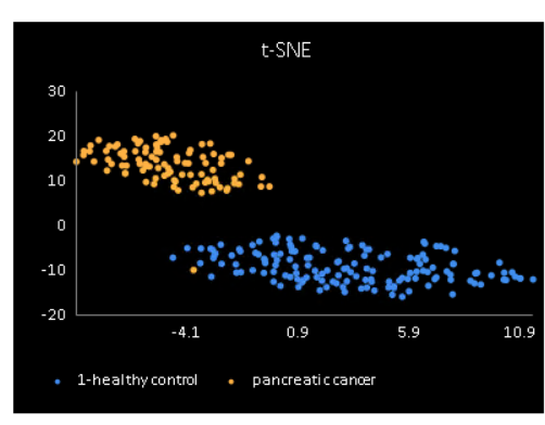
  7. Click on to display the t-SNE plot.

    Extra features:

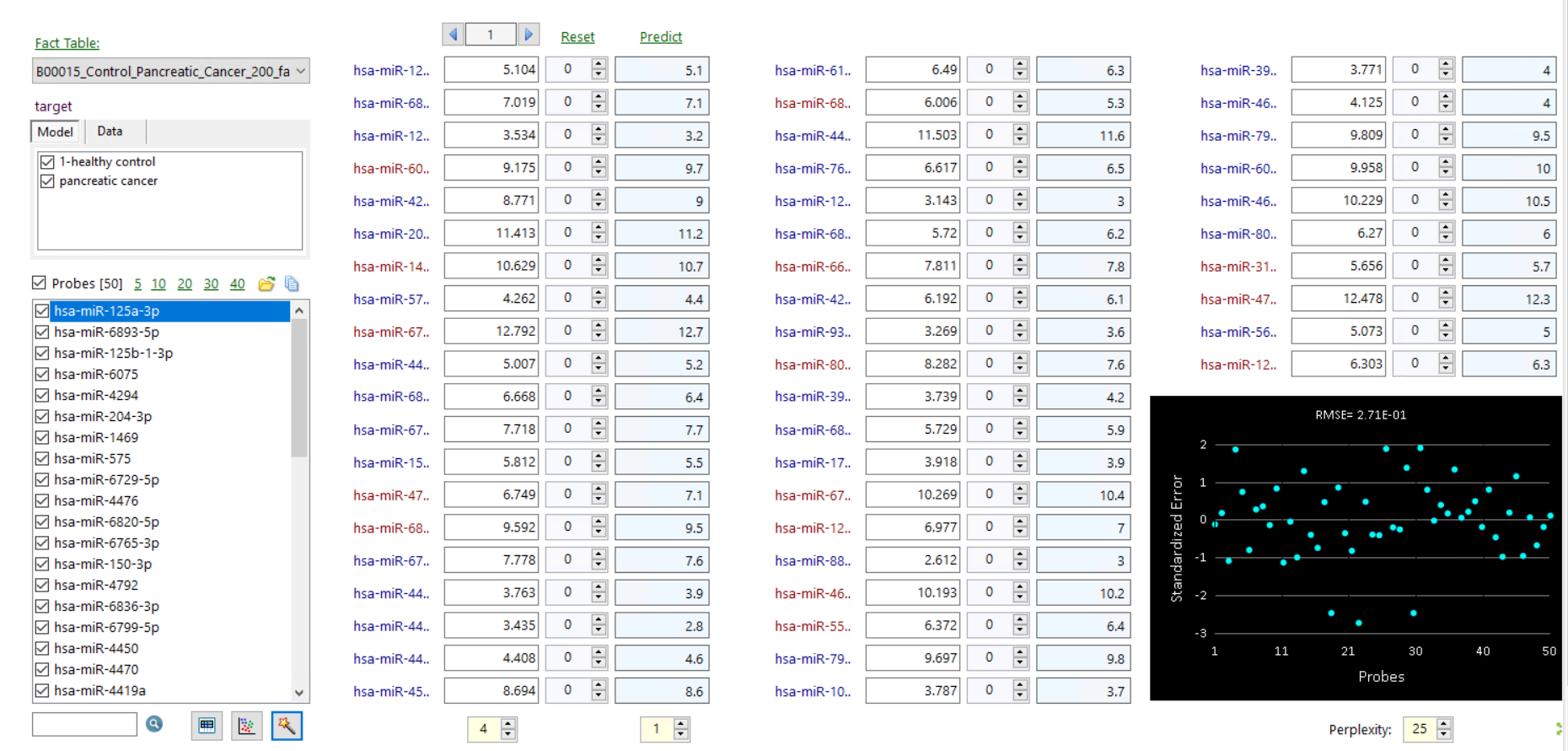
  • Click on row changer to use different samples for simulation.
  • Click on Reset hyperlink to clear the changes.
  • Make changes to the sample data using the reset option in between actual and predicted values and see how the predicted values change on the fly.
  • Click on Predict hyperlink to
  • Change the number of decimals to the right that should be considered in both actual and predict values using number option at the bottom of the screen.
  • Perplexity gives a guess on how many neighbors are nearby. Lower the perplexity value when the data points are low.
  • Click on to show the plots in full screen.

Dataset

  1. Click on the to get the dataset used for building simulation models.
  2. Click on to run the modified query.
  3. Click on to save the dataset to local computer.
  4. Click on to get the aggregate of the data.